Monetary Policy and the Transmission of Interest Rates

Public working draft: This AI-assisted feasibility draft is open for coauthor revision. Empirical descriptions, causal claims, policy judgments, and figure rights remain subject to human review. Chapter 11 separately covers the Federal Reserve System and operating framework.
Central question: How can one Federal Reserve policy decision change borrowing, spending, employment, and inflation—and why do the effects arrive unevenly and with uncertain lags?
By the end of this chapter, you should be able to: distinguish a policy decision from its operational implementation; trace current and expected policy rates into market yields and credit terms; calculate how a mortgage rate changes a feasible payment; compare effects on borrowers, savers, renters, and owners; use simple present-value reasoning for investment; explain expectations, credit, and exchange-rate channels; distinguish the effective lower bound from ordinary implementation; and evaluate a monetary-policy episode without reading chronology as proof.
10.1 From a Fed announcement to a homebuyer’s budget
Imagine a first-time homebuyer in early 2022. She has saved a down payment, compared neighborhoods, and decided that principal and interest of about $1,500 per month would fit her budget. A lender’s quoted mortgage rate then rises. The house has not changed. Her wage has not changed. Yet the combination of price and monthly payment she can afford has changed.
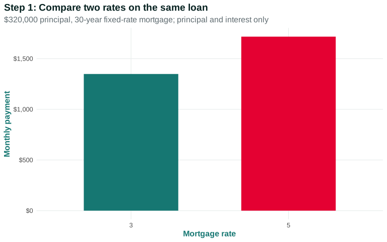
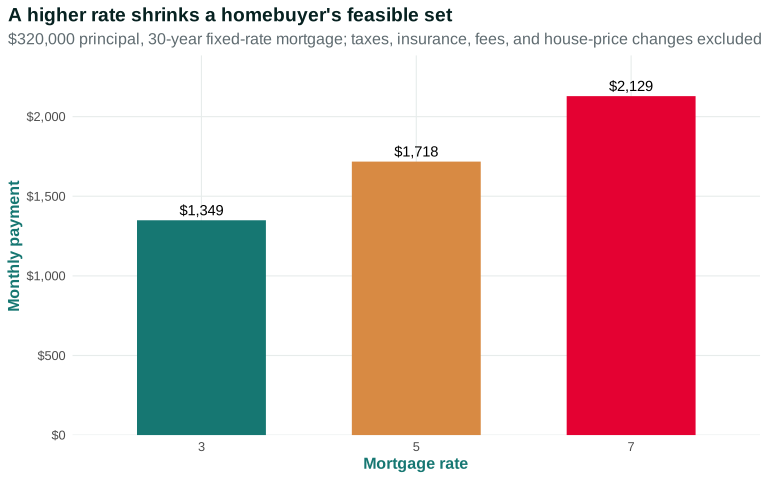
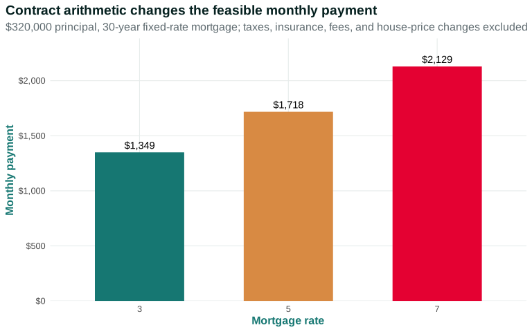
Begin with the household’s contract rather than the central bank. Figure 10.1 holds a $320,000 principal and 30-year term fixed while changing one rate. The bars therefore answer a bounded question: what monthly principal-and-interest payment is required when only the mortgage rate changes?
Open the live step-by-step figure
At 3 percent, the monthly payment is about $1,349. At 5 percent it is about $1,718, and at 7 percent about $2,129. Compare the 3 and 7 percent bars: the same principal requires roughly $780 more each month. A household whose payment ceiling is fixed must bring a larger down payment, buy a less expensive home, or delay. The arithmetic changes the feasible set; it does not tell us which choice the household will make.
The figure excludes taxes, insurance, fees, down payments, lender qualification rules, and house-price changes. That is its strength and limitation: it isolates one contract effect. Sellers may lower prices, incomes may change, and lenders may tighten standards at the same time. A transparent calculation is not yet a forecast of the housing market.
Now ask where the quoted mortgage rate comes from. The Federal Open Market Committee does not set it. The committee announces a target range for an overnight interest rate in a market among financial institutions. A 30-year mortgage instead bundles expected future short rates, longer-term Treasury yields, inflation expectations, prepayment risk, credit risk, lender costs, competition, and fees. Understanding monetary policy means tracing this chain, not drawing an arrow from “Fed” directly to “mortgage.”
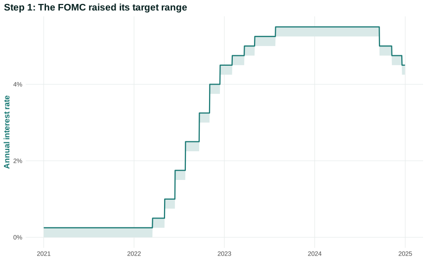
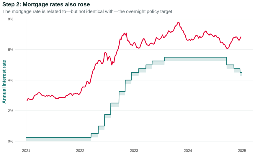
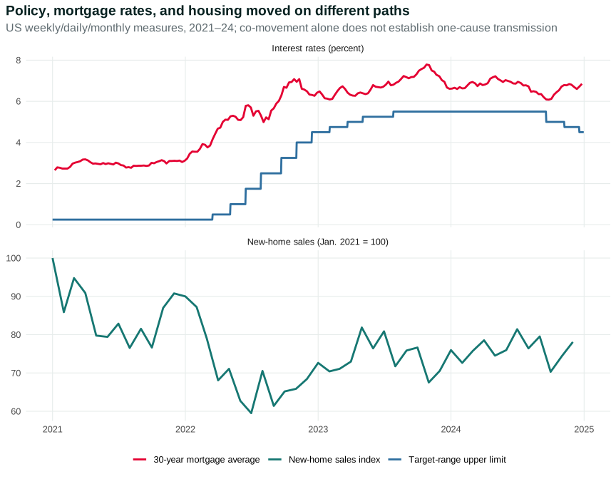
Figure 10.2 begins with the federal funds target range. The lower and upper limits are annual rates, even though the target concerns overnight borrowing. The second step adds a national weekly average 30-year fixed mortgage rate. The summary adds monthly new single-family home sales, indexed so January 2021 equals 100.
Open the live step-by-step figure
Read each panel before comparing them. The target range is daily, the mortgage average weekly, and home sales monthly at a seasonally adjusted annual rate before indexing. The index reports relative movement, not a count of houses. The lines can turn at different dates because markets anticipate policy and respond to other news.
The chronology is consistent with a transmission story: tighter policy, higher borrowing costs, and weaker interest-sensitive activity. It is not a complete causal estimate. Housing supply, construction cost, household income, remote work, demographic demand, mortgage spreads, and expectations also changed. Policy itself responds to inflation and employment, creating reverse causality.
The hook has now established one exact link and one uncertain chain. The payment formula tells us what a quoted rate does to a specified contract. The time series show that policy rates, mortgage rates, and housing activity moved on different schedules. The broader central question is how one Federal Reserve decision can change borrowing, spending, employment, and inflation—and why the effects arrive unevenly and with uncertain lags.
Questions
Review the live step-by-step figure
Question 10.1. What does Figure 10.1 establish?
- All housing changes were caused only by the Fed
- Policy, mortgage, and housing measures moved on different paths
- Mortgage and policy rates are identical
- The three series have one frequency
Exercise
Three moving measures
Use Figure 10.1 to compare units, timing, and one causal claim the chronology cannot establish.
The model solution is available in the restricted instructor materials.
10.2 The central bank’s goals and policy decision
Congress has assigned the Federal Reserve goals including maximum employment and stable prices. Policymakers observe current data, build forecasts, assess risks, and select a policy stance: how supportive or restrictive financial conditions are intended to be relative to economic circumstances. Chapter 11 explains who votes and how the decision is implemented. Here we focus on what the choice is trying to accomplish.
The goals cannot be read from one current statistic. Inflation is measured with a delay and includes past price changes. Employment data are revised. Interest-rate changes operate over time. The committee therefore makes a forecast-based decision under uncertainty. It asks how demand, supply, expectations, financial stability, and policy already in the pipeline may evolve.
If aggregate demand is weak and inflation pressure is low, a lower policy-rate path can encourage interest-sensitive spending and reduce debt-service pressure on new borrowers. If demand is strong and broad inflation is persistent, a higher path can restrain spending and labor-market pressure. But Chapter 8 showed why an adverse supply shock is difficult: tighter demand can limit propagation while imposing additional output and employment losses; easier policy cannot create missing energy or semiconductors.
“Maximum employment” is not a single fixed unemployment number. People enter and leave the labor force, matching changes, discrimination and bargaining institutions matter, and labor-market indicators can disagree. “Stable prices” does not mean every price is unchanged. Relative prices must change when scarcity and preferences change. The policy concern is the path of the general price level and inflation expectations, not preventing all individual increases.
Policy involves risk management. Waiting for complete proof can allow inflation expectations or unemployment to worsen. Acting aggressively can create unnecessary recession or financial stress. Policymakers can disagree because their forecasts, values, and estimates of transmission differ—not only because one side understands economics and the other does not.
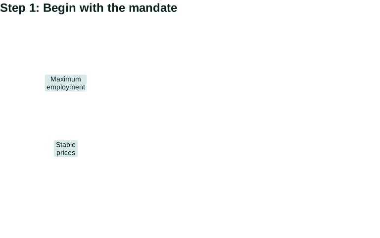
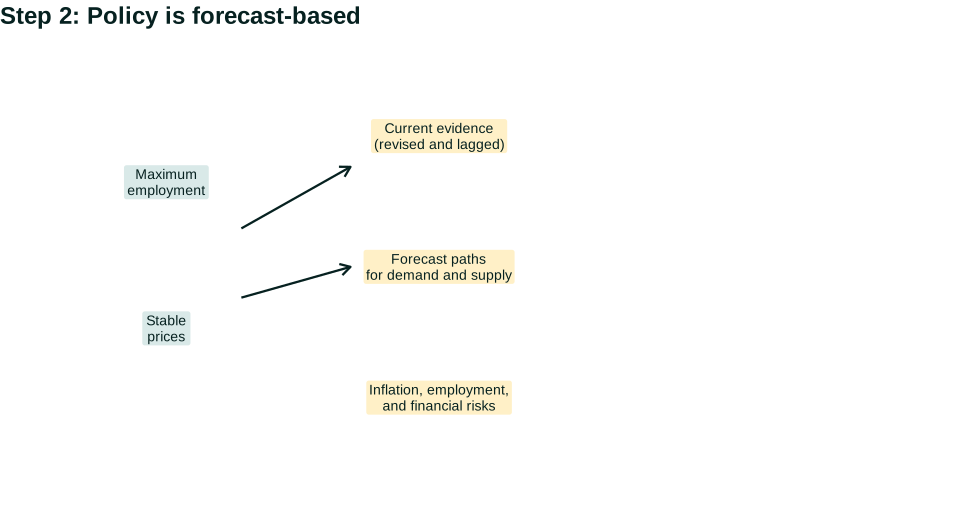
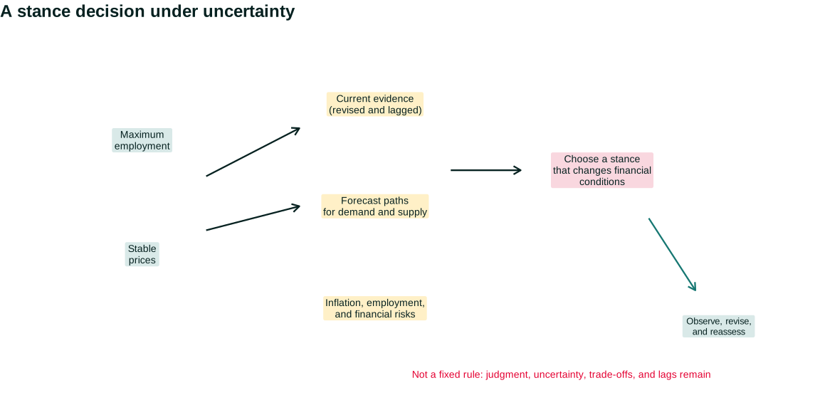
Figure 10.3 makes the decision process visible without pretending it is a mechanical rule. The first step identifies the two mandated goals. The second adds forecasts and risks because policy affects future conditions with lags. The summary adds the stance decision and the commitment to reassess as evidence changes.
Open the live step-by-step figure
Read the dashboard from left to right. The mandate does not produce a unique setting. Policymakers interpret noisy indicators, compare possible future paths, and judge asymmetric risks. A rate increase can reduce demand pressure but cannot produce oil or repair a supply chain. A rate cut can support demand but cannot guarantee that cautious lenders or pessimistic firms will respond. The decision changes one important constraint; it does not command the outcome.
This actor-and-chain route also follows a teaching lesson emphasized by Federal Reserve educators Scott Wolla and Tim Lloyd: policy is transmitted through market rates and the spending decisions of consumers and producers. For this chapter, that simple sequence is a starting scaffold. The sections that follow add the maturities, spreads, balance sheets, access, and feedbacks needed to make it accurate for first-year college students. St. Louis Fed transmission teaching scaffold
An announced target range is the decision. The Board and Federal Reserve Banks then use an ample-reserves operating system to keep overnight rates consistent with it. Chapter 11 will teach administered rates, reserves, and the balance sheet. Keeping implementation separate prevents a conceptual error: operational success in steering one overnight rate does not guarantee the desired effects on mortgage rates, investment, employment, or inflation. Federal Reserve current policy description
To understand those effects, follow the price of credit outward through maturities and risk.
Questions
Question 10.2. Why is monetary policy forecast-based?
- Employment and inflation respond before any decision
- Policy has lags and current data are incomplete
- The Fed observes the future
- Supply shocks create no trade-off
Exercise
Shock diagnosis
Compare the monetary-policy problem created by a demand expansion with that created by an adverse supply shock.
The model solution is available in the restricted instructor materials.
10.3 From the policy rate to market interest rates
The policy interest rate is a short-term rate used to signal and implement the stance of monetary policy. Households and firms borrow at many other rates. A lender choosing the price of a five-year loan cares about expected short rates over those years, expected inflation, the chance of default, funding costs, collateral, administrative expense, and profit. TE 2.0 monetary-transmission sequence
Suppose a one-year Treasury yield can be thought of, roughly, as the expected average overnight rate plus compensation for holding a longer asset. If market participants learn today that the policy path will probably be higher next year, a one-year yield can rise immediately even before the current target changes. Conversely, a current rate increase can be followed by falling long yields if it convinces investors that inflation will decline and later policy rates will be lower.
A risk spread is the difference between a borrowing rate and a safer benchmark with a similar maturity. Spreads can widen during stress because default risk, uncertainty, market liquidity, and lender balance sheets change. A central-bank cut can therefore coexist with higher rates for some risky borrowers. Transmission is not one-for-one.
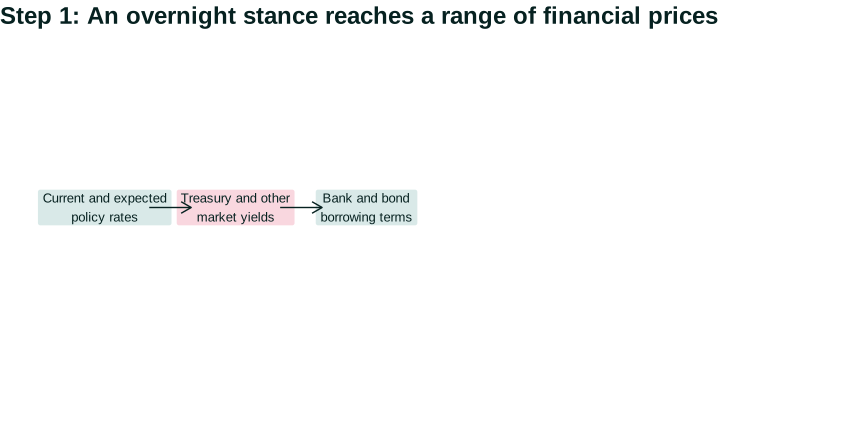
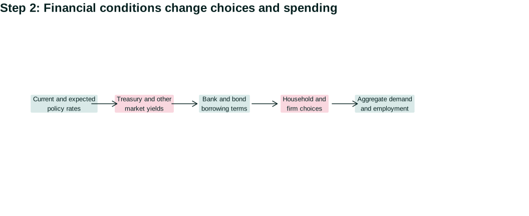
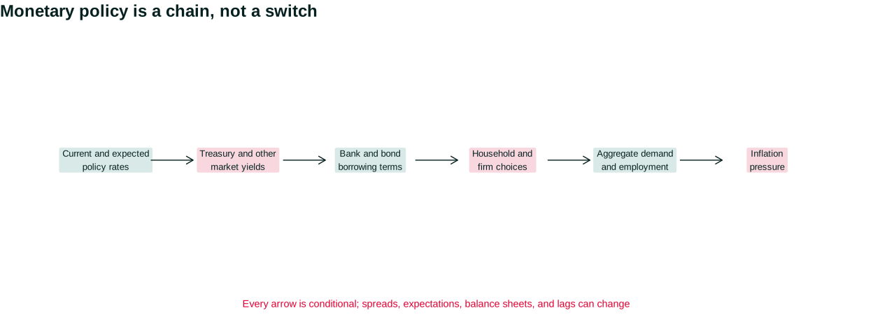
Figure 10.4 organizes the links.
Open the live step-by-step figure
Each arrow is an empirical question. Did expected policy move? Which maturity responded? Did bank funding or risk spreads change? Were creditworthy borrowers willing to borrow? Did spending respond, or were households repairing balance sheets and firms pessimistic about sales? Did extra demand raise quantities or prices? A model that replaces all these rates with one (r) is a useful shorthand only after students understand what it compresses.
Inflation expectations connect nominal and real rates. If a nominal borrowing rate is 6 percent and expected inflation is 3 percent, the expected real rate is approximately 3 percent. If expected inflation falls to 2 percent while the nominal rate remains 6, the expected real rate rises to about 4 percent. A nominal rate held constant can therefore become more restrictive.
Financial markets respond quickly; contracts and production respond more slowly. That difference helps explain why policy announcements move yields within minutes while employment and inflation may take many months. The next two sections open the household and firm decision boxes.
Questions
Review the live step-by-step figure
Question 10.3. A borrowing spread can widen when…
- risk and lender balance-sheet stress rise
- all borrowers become identical
- maturity ceases to exist
- accounting requires it to be zero
Exercise
Trace a spread
Explain why a policy-rate cut can coexist with a higher borrowing rate for a risky firm.
The model solution is available in the restricted instructor materials.
10.4 Household transmission
Households differ by age, income, wealth, debt, tenure, credit score, location, family obligations, disability, and citizenship. “Higher rates reduce consumption” is therefore a summary of several opposing mechanisms.
For a household considering a new car or home, a higher borrowing rate raises the payment for a fixed purchase price. It can postpone the purchase, lower the amount borrowed, shift demand toward a cheaper product, or require a larger down payment. These are substitution and cash-flow effects on a new contract.
Existing contracts matter. A homeowner with a 30-year fixed-rate mortgage does not see the required payment change when market rates rise. The same household may become reluctant to move because selling would mean giving up the old rate. A borrower with an adjustable-rate mortgage, credit-card balance, or new lease can face faster payment changes. A renter can be affected indirectly through landlord financing, construction, and housing supply.
Savers can gain interest income. A retiree holding short-term deposits or Treasury bills may spend more when rates rise. A young indebted household may cut spending. The aggregate effect depends on whose income changes and how each responds. Because borrowers and savers have different propensities to spend, redistribution is part of transmission rather than an afterthought.
Asset prices and collateral create another channel. Higher discount rates can lower the present value investors place on future payments, reducing some bond, stock, or property prices. Homeowners may feel less wealthy; lenders may see less collateral; leveraged investors may sell. Yet asset prices also reflect expected profits, rents, risk, and news about the economy, so a policy announcement need not move all assets in one direction.
Credit access is not just a rate. A lender can reject an application, require more collateral, shorten maturity, or tighten documentation. Discrimination and unequal inherited wealth mean similarly situated households may face different choices. A policy designed around an “average borrower” can miss who actually loses access.
Follow five households through one rate increase
Return to a two-percentage-point increase in market borrowing rates. Household A is applying for a first mortgage. The higher quoted payment reduces the maximum principal consistent with the lender’s debt-to-income rule. The household can buy a cheaper home, increase its down payment, delay, or leave the market. If many prospective buyers delay, sellers and builders may lower prices, reduce construction, or wait.
Household B bought a home several years ago with a fixed-rate mortgage. Its required principal-and-interest payment does not change. But moving now would require a new mortgage, so the household may remain in a house that no longer fits its job or family needs. This “lock-in” reduces listings as well as demand. A lower volume of transactions does not necessarily mean every owner is financially distressed.
Household D carries a variable-rate credit-card balance. Its required interest payment rises quickly, leaving less cash for groceries, recreation, or debt repayment. If it misses payments, its credit score and future access can deteriorate. The same rate rise reaches this household faster than Household B.
Household E is a retiree with Treasury bills and bank deposits but little debt. Interest income rises as assets roll over. It may spend some of that income. Whether aggregate consumption falls depends partly on the relative size and spending response of indebted and asset-owning households. Netting “borrowers lose, savers gain” in dollar terms is not enough.
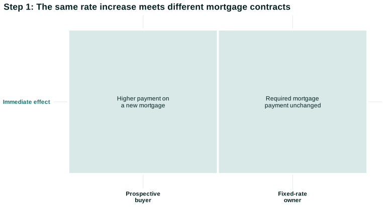
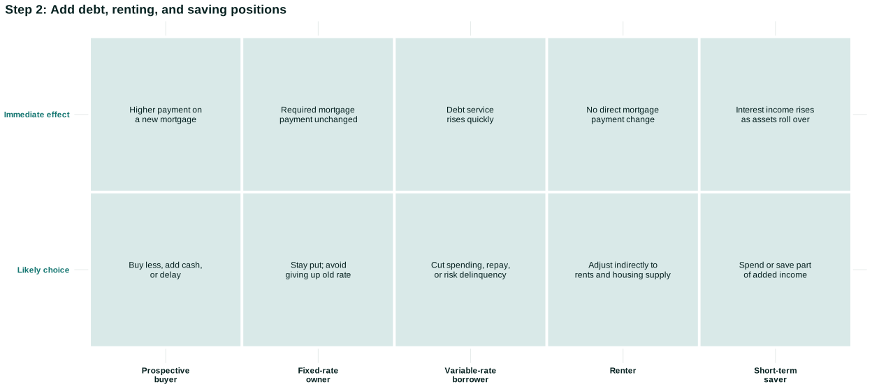
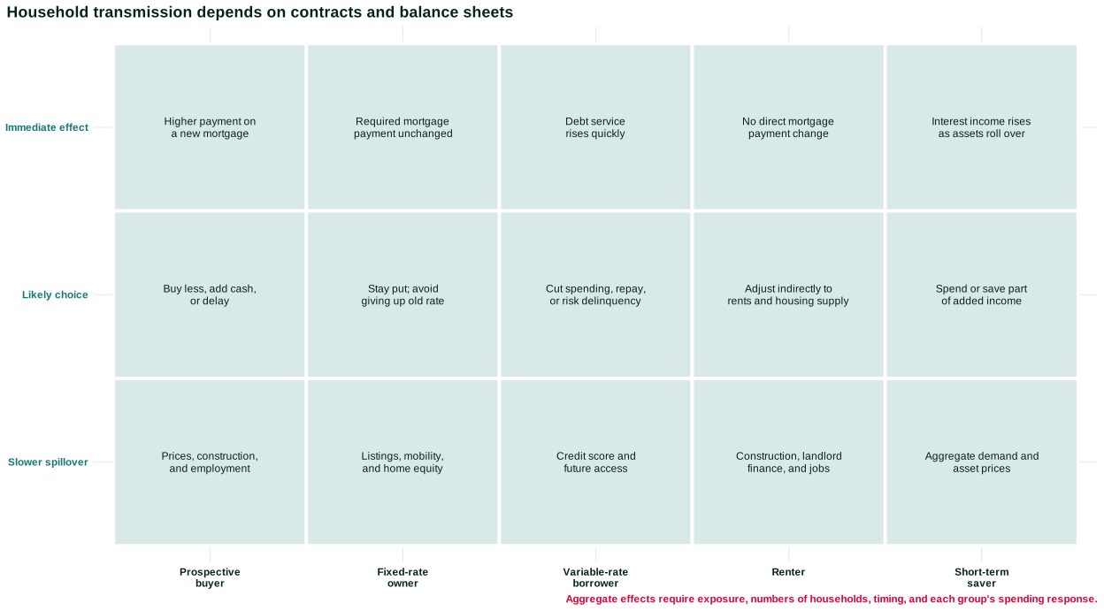
Figure 10.5 holds the market-rate increase fixed and compares the contracts and balance sheets. The first step separates a prospective borrower from an existing fixed-rate borrower. The second adds a variable-rate borrower, renter, and saver. The summary names the immediate cash-flow effect, likely adjustment, and slower spillover for each case.
Open the live step-by-step figure
The rows are not five separate economies. They coexist, so aggregation requires their relative numbers, dollar exposures, and spending responses. A fixed-rate mortgage delays payment pass-through for the existing loan, but it does not remove the owner from monetary transmission: moving, refinancing, home equity, employment, and asset prices remain possible routes. Recent Federal Reserve research using mortgage and credit data finds that new borrowing by households not usually treated as marginal buyers can make mortgage debt-service transmission build over time. The empirical magnitude belongs to that study and period; the durable lesson is to follow flows of new contracts as well as the stock of old ones. Federal Reserve mortgage-payment research
Wealth positions reflect past institutions. Redlining, exclusion from subsidized mortgages, unequal family transfers, segregation, labor-market discrimination, and place-based house-price changes shape who owns assets and who borrows. The transmission mechanism therefore inherits historical class and racial inequalities even when the policy rate is formally uniform.
There is also a time dimension. New mortgage applications react within weeks; construction employment responds after projects change; rents reset over months; fixed-rate debt can remain insulated for years. Surveying households immediately after an announcement may find little spending response even when later housing supply changes substantially. A lag is not evidence that the channel does not exist.
Students should resist turning these cases into fixed signs. Higher deposit income can be offset by falling asset prices. A renter can benefit from lower demand or be harmed by less construction. A homeowner can enjoy a low payment while losing mobility. The method is to identify the balance sheet, contract, feasible alternatives, and adjustment horizon before aggregating.
The mortgage example illustrates the Trade-offs and opportunity costs principle. Higher rates can restrain housing demand and inflation pressure, but they make entry harder for new buyers and can slow construction. Existing owners with fixed low rates are partly insulated, while renters may not benefit if supply falls. Distribution and stabilization travel through the same contract structures.
Household spending is one component of aggregate demand. Firm investment and hiring provide another.
Questions
Review the live step-by-step figure
Question 10.4. Who is most directly insulated from an immediate market-rate rise?
- A new mortgage applicant
- A homeowner with an existing fixed-rate mortgage
- A variable-rate borrower
- A firm seeking a new loan
Exercise
Household positions
Compare a new buyer, fixed-rate owner, adjustable-rate borrower, renter, and saver after the same rate increase.
The model solution is available in the restricted instructor materials.
10.5 Firm transmission
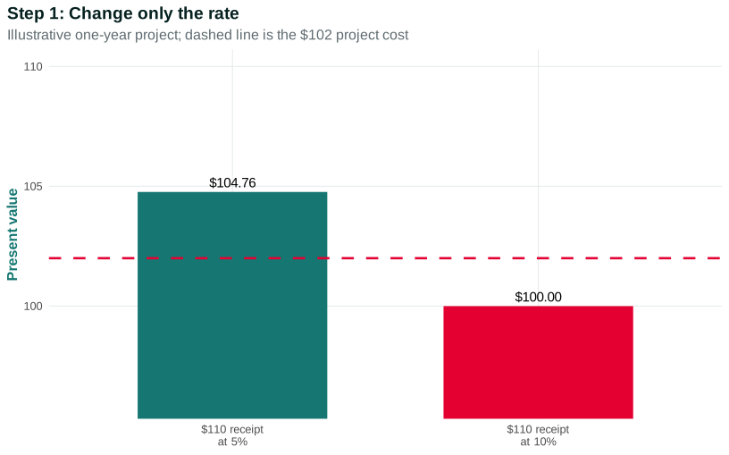
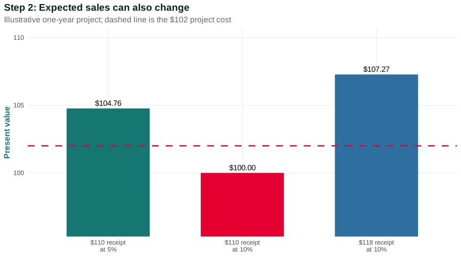
A firm considering a machine compares a cost today with expected future revenue and cost savings. The simplest present value asks how much a future payment is worth today given an interest rate. If a project pays $110 one year from now and the relevant rate is 10 percent, its present value is $100. At 5 percent it is about $104.76. A higher discount rate lowers present value, other things equal.
This arithmetic is not a complete investment model. The relevant rate includes risk. Future cash flow is uncertain. Managers may value strategic position, worker safety, environmental effects, or control, not only one-year profit. Firms can finance with retained earnings, bank loans, bonds, equity, supplier credit, or owner wealth. Their response to policy differs.
Consider two firms. A profitable technology company with cash may not need a loan, but higher rates can lower customer demand and asset valuations. A small restaurant relying on a variable-rate bank loan experiences an immediate cash-flow increase. A manufacturer contemplating a ten-year plant cares about long yields, expected sales, taxes, and capacity. One policy decision changes their feasible sets differently.
Expected demand can dominate financing cost. If a rate cut occurs because policymakers foresee recession, firms may still cancel projects. If expansion raises expected sales, investment can increase despite moderately higher rates. This is an accelerator mechanism: investment responds to expected output as well as its financing price.
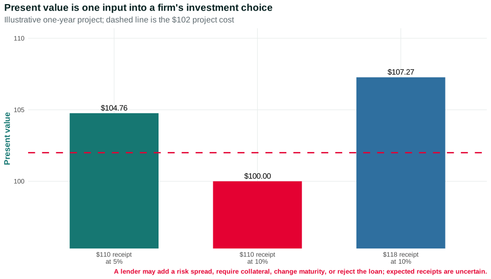
Figure 10.6 begins with the transparent one-year project from the Math Extension. Step 1 changes only the financing rate. Step 2 changes expected receipts as well. The summary adds the lender’s risk spread and collateral decision, making clear why present-value arithmetic is one input rather than an observed causal estimate of investment.
Open the live step-by-step figure
Compare the first two bars while holding $110 fixed: the rate change alone moves present value from about $104.76 to $100. Then compare the second and third bars: with the rate still at 10 percent, expected receipts of $118 raise present value to about $107.27. A project costing $102 switches from rejection to acceptance in this illustration. The changed condition is expected sales, not a reversal of the discount-rate logic.
A project’s rate is not the policy rate
Suppose a small manufacturer can buy a $1 million machine expected to reduce labor and energy costs over ten years. A simple textbook might discount those savings using the policy rate. The firm cannot borrow at that rate. Its loan offer includes a benchmark yield, a spread for default risk, bank costs, collateral requirements, and possibly a floating-rate provision. The owner may also be required to guarantee the debt personally.
When the policy path rises, the benchmark can rise. If the economy also weakens, the lender may widen the spread because expected default increases. The loan rate can therefore rise by more than the policy rate. If inflation uncertainty declines and the firm’s order book remains strong, the spread or long yield may instead offset part of the increase. Observed loan pricing combines several links.
The machine affects workers as well as owners. It may increase productivity, reduce dangerous tasks, eliminate some jobs, require new training, or intensify monitoring. A present-value calculation based on firm cash flow does not measure all social benefits and costs. Taxes, bargaining, worker voice, and labor standards determine how productivity gains are shared.
Financing structure changes exposure. A large corporation can issue a bond with a fixed coupon and maturity. A startup may rely on equity whose valuation responds to discount rates and risk appetite. A family business may use a home as collateral. A nonprofit hospital may issue tax-exempt debt while facing regulated reimbursement. “Investment demand” aggregates institutions with different authority and risk.
Inventories can respond before fixed investment. Higher carrying costs make unsold goods more expensive to finance. Firms may reduce orders, discount products, or run leaner inventories. Suppliers then experience fewer sales. During a supply disruption, however, firms may deliberately hold more inventory as insurance despite higher rates. Goals and constraints can reverse the usual sign.
Hiring decisions connect financial and product markets. A firm anticipating weaker demand may stop posting vacancies before cutting production. Lower vacancy pressure weakens workers’ outside options from Chapters 2–4. Wage growth can slow; unit costs and price adjustments may slow later. This is one route from monetary restraint to inflation, but it is neither instantaneous nor costless.
Business failure is a nonlinear response. A modest cash-flow increase may be manageable for a firm with reserves; the same increase can push a leveraged firm into default. When many firms are close to a threshold, a small rate change can produce a large employment effect. Average debt ratios can hide that tail risk.
Policy evaluation should therefore examine borrowing volumes, applications and rejection, loan terms, spreads, investment, vacancies, and firm exit—not only a single average interest rate. Each measure locates a different link in the transmission chain.
Bank balance sheets can amplify changes. Falling collateral values or rising defaults can cause lenders to tighten standards. Borrowers cut investment and employment; income falls; defaults rise; standards tighten further. The Aggregation and feedback principle makes credit both a transmission channel and a possible amplifier.
Employment changes after several decisions. Firms may first reduce vacancies, overtime, or temporary work, then delay hiring or lay off workers. Workers with weaker bargaining power and fewer savings bear more risk. Monetary restraint is therefore not a painless movement along an inflation curve. It changes concrete employment and financing opportunities while attempting to reduce aggregate demand pressure.
For a payment (F) one year from now and rate (r), (PV=F/(1+r)). A project costing $102 today and paying $110 next year has positive net present value at 5 percent because (110/1.05 ), but negative net present value at 10 percent because (110/1.10=100). The example changes only the rate. In practice, expected cash flow and risk may change at the same time.
Questions: Which project decision changes between the two rates? What additional information would you need before treating this arithmetic as a forecast of actual investment?
Market rates and domestic spending are not the only routes. Expectations, credit quantities, and international asset choices matter too.
Questions
Question 10.5. Holding a future payment fixed, a higher discount rate…
- raises present value
- leaves present value unchanged
- lowers present value
- proves investment falls by the same amount
Exercise
Investment arithmetic
Calculate present value under two rates, then identify two behavioral facts omitted by the arithmetic.
The model solution is available in the restricted instructor materials.
10.6 Expectations, credit, and the exchange rate
Central-bank communication can affect choices because contracts depend on the expected future path of rates. A statement, forecast, or press conference can move yields even when the current target is unchanged. This does not mean words work independently of credibility. Market participants ask whether future policymakers will act as described and how new data will change the path.
An announcement contains several kinds of news at once. It reports a policy decision, but it can also reveal the central bank’s assessment of the economy. Suppose the committee cuts rates more than markets expected. Investors might lower long yields because expected short rates fell. Or long yields could rise if the decision reveals a stronger outlook or changes perceived inflation risk. Measuring the “surprise” requires knowing what was expected immediately beforehand.
Forward guidance can be calendar-based—rates are described as likely to remain low until a date—or condition-based—policy depends on employment and inflation. Calendar language is simple but may become inappropriate as conditions change. Conditional language is adaptable but requires the public to understand how data affect decisions. Neither removes uncertainty.
Communication reaches unequal audiences. Large financial institutions process statements and projections instantly. Households may learn through news headlines, lenders, or changing payments. Technical language can obscure the policy’s distributive stakes. Transparency is not only publishing more documents; it includes explaining what decisions do and do not control.
Expectations also affect inflation. If firms and workers expect inflation to remain high, they may build larger price and wage changes into contracts. A credible tightening can reduce expected inflation and long-term nominal yields. But credibility is not a free resource or a command. It emerges from institutions, past behavior, evidence, communication, and political legitimacy.
Credit quantity can change independently of posted rates. During stress, banks and capital markets may ration credit because borrower risk is difficult to price or lender capital is constrained. A small firm can face “no loan” rather than a loan two percentage points more expensive. Facilities that support market functioning can therefore affect transmission even when the policy stance is described by an interest rate.
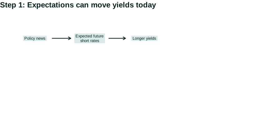
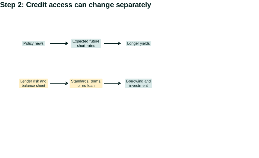
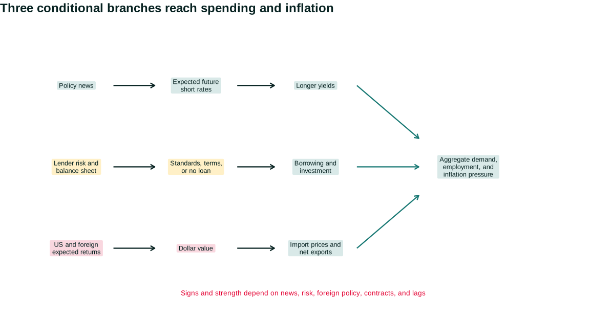
Figure 10.7 places three conditional branches beside one another. Expected future policy changes yields today. Lenders can change approval standards and contract terms as well as rates. International investors can change the dollar’s value, import prices, and net exports. The branches later meet in aggregate demand and inflation pressure, but they need not move with equal strength or even the same sign on announcement day.
Open the live step-by-step figure
The Senior Loan Officer Opinion Survey helps locate the credit branch. It asks banks separately about approval standards, contract terms, and loan demand. Those are not synonyms. Standards govern whether an application is approved; terms govern price, size, maturity, covenants, or collateral conditional on approval; demand records borrowers’ reported interest in credit. A fall in lending can reflect any combination, so one loan-volume series cannot identify the mechanism. Federal Reserve SLOOS definitions
International investors compare expected returns across currencies. A higher expected US interest-rate path can increase demand for dollar assets and contribute to dollar appreciation, other things equal. A stronger dollar makes imports cheaper in dollars and US exports more expensive to foreign buyers. Net exports can fall, reducing aggregate demand; cheaper imports can reduce some inflation pressure.
The exchange-rate result is conditional. Expected future policy, global risk, foreign rates, trade invoicing, hedging, and geopolitical news also matter. In a global “flight to safety,” the dollar can appreciate even when US rates fall. Chapter 14 will build the open-economy mechanism in depth.
These channels show the Interdependence principle. One country’s policy changes asset prices, exchange rates, debt service, and demand elsewhere; foreign responses feed back to US production and inflation. Borrowers with dollar debt outside the United States may be exposed even when their domestic income is not in dollars.
Ordinary rate cuts have a limit. When very short safe nominal rates approach their effective lower bound, further conventional reductions become constrained.
Questions
Question 10.6. A stronger dollar can, other things equal…
- make imports cheaper and reduce net exports
- guarantee exports rise
- eliminate global feedback
- prove US rates rose
Exercise
Dollar channel
Trace an appreciation from international asset demand through imports, exports, aggregate demand, and inflation.
The model solution is available in the restricted instructor materials.
10.7 The effective lower bound and balance-sheet policy
The effective lower bound is the region in which the central bank has limited room to reduce its conventional short-term nominal policy rate. The bound is “effective,” not mechanically zero: slightly negative rates have existed in some countries, but cash, financial institutions, and market functioning limit how far they can fall.
If expected inflation also declines, the expected real rate can remain high even when the nominal rate is near zero. Suppose the nominal rate is 0.5 percent and expected inflation falls from 2 percent to zero. The approximate expected real rate rises from −1.5 to 0.5 percent. Weak demand can therefore coexist with little conventional room to cut.
Central banks can influence broader conditions through communication about future rates, lending facilities, and purchases of longer-term securities. Large-scale asset purchases exchange one kind of government-linked asset for another and can affect longer yields, risk premia, liquidity, and portfolios. Their effects are not identical to cutting the overnight target, and estimates vary by episode and market condition.
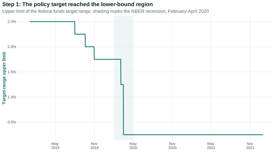
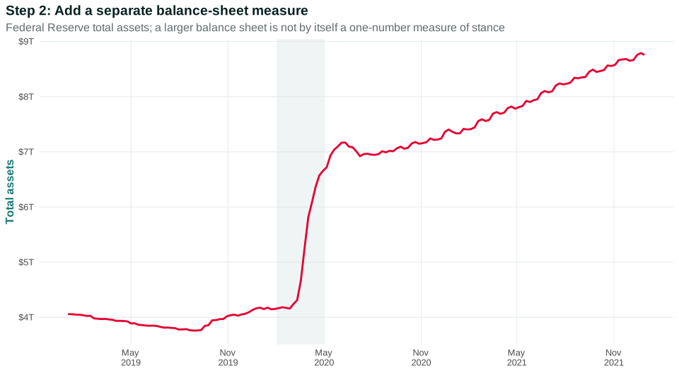
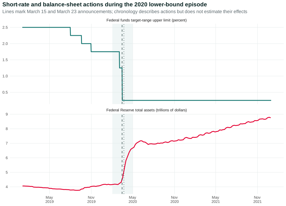
Figure 10.8 uses the 2020 shock to separate two actions. Step 1 shows the upper limit of the federal funds target range falling into the lower-bound region. Step 2 adds total Federal Reserve assets, a broad balance-sheet measure, on its own axis. The summary marks the March policy and purchase announcements and the NBER recession interval. It does not label the balance-sheet increase as a one-number measure of stance.
Open the live step-by-step figure
On March 15, the FOMC announced a target range of 0 to 0.25 percent and directed purchases of at least $500 billion in Treasury securities and $200 billion in agency mortgage-backed securities over coming months. On March 23, it shifted to purchases in amounts needed to support market functioning and transmission. Those official statements identify actions and stated purposes. The plotted co-movement does not by itself estimate their effects on yields, lending, employment, or inflation. Federal Reserve 2020 lower-bound actions
Balance-sheet policy must be separated from routine implementation. In the current ample-reserves framework, the Federal Reserve uses administered rates to steer the federal funds rate while reserve balances are abundant. A large balance sheet does not by itself tell us whether the policy stance became easier or tighter on a particular day. Chapter 11 will show the balance sheets and operational tools.
Nor should asset purchases be described as mechanically multiplying bank reserves into a fixed quantity of household loans. Banks make lending decisions based on profitable opportunities, borrower creditworthiness, capital, liquidity, funding, and regulation. Households do not borrow merely because banks hold additional reserves. The old mechanical money-multiplier story mistakes an accounting relationship for a behavioral law.
Lower-bound tools have distributional and political consequences. Asset-price changes affect owners and prospective buyers differently. Emergency lending can stabilize employment and payments while creating questions about eligible institutions, collateral, losses, and democratic authority. Those institutional questions belong at the center of Chapter 11, not in a technical footnote.
We can now return to the 2022–24 evidence and practice making a mechanism-based, appropriately cautious claim.
Questions
Question 10.7. Why avoid a mechanical money-multiplier story?
- Bank lending is a behavioral choice shaped by creditworthiness, capital, liquidity, and demand
- Reserves are household deposits
- Every reserve dollar legally requires a fixed loan multiple
- Balance sheets never matter
Exercise
Lower-bound distinction
Explain why asset purchases and routine ample-reserves implementation should not be treated as the same policy action.
The model solution is available in the restricted instructor materials.
10.8 Trace one policy episode
Start with the policy problem. Inflation had risen, but demand pressure, supply constraints, expectations, wages, margins, and global shocks all contributed in changing proportions. A mechanism-based account should not claim the Fed directly chose the observed inflation or unemployment rate.
Next trace the indicators. The target range rose. Mortgage rates also rose, but at different dates and by different amounts. New-home sales weakened relative to early 2021, while month-to-month variation remained. The evidence is consistent with interest-sensitive housing transmission. It is not enough to isolate the Fed’s effect from supply, income, expectations, and risk.
To see the identification problem, imagine inflation data arrive stronger than expected on Monday. Mortgage rates rise because investors anticipate tighter policy. The FOMC raises the target on Wednesday, exactly as anticipated, and mortgage rates barely move that afternoon. A same-day comparison would conclude policy had no effect; a monthly comparison might assign Monday’s market movement to Wednesday’s announcement. Both miss anticipation.
Now imagine financial stress widens mortgage spreads while the Fed cuts its target. Mortgage rates could still rise. Reading the two lines alone might say easing “caused” higher mortgage rates, when both were responses to stress through different links. A causal study tries to isolate an unexpected policy component from information about the economy and other shocks.
Even after identification, the estimated effect is distributed over time. Housing applications may react quickly, construction later, employment after that, and measured shelter inflation with still longer lags. Inflation indexes use contracts and samples that update gradually. Asking whether policy “worked” after one month can be meaningless.
The counterfactual also matters for welfare. If inflation falls after tightening, it might have fallen anyway as supply constraints eased. If unemployment rises, it might have risen more without restored price stability—or less without tighter demand. Policy evaluation compares plausible paths, not observed before-and-after values.
Carry the evidence tests from Chapter 8 forward. If goods quantities rebound while prices slow as bottlenecks clear, supply normalization is doing work. If vacancies, spending, wage growth, and price pressure weaken together, demand transmission is plausible. If longer-run expectations remain stable, an expectations-deanchoring story is weakened. Multiple mechanisms can operate together without making causal judgment arbitrary.
Distribution is part of the episode. New borrowers and construction workers experience restraint differently from holders of interest-bearing assets. Lower inflation benefits households whose wages or benefits lag prices, yet unemployment risk is concentrated. Asset-price changes affect wealth holders and pension funds. An aggregate success can contain severe losses for particular groups; an aggregate cost can accompany valuable risk reduction.
Finally separate implementation from transmission. The effective federal funds rate can remain inside the target range throughout the episode—evidence that the operating framework controlled its immediate rate—while mortgage spreads, lending standards, and spending behave unexpectedly. Chapter 11 explains that operational achievement. It should not be confused with proof about the entire macroeconomic chain.
A careful evaluation therefore asks four different questions. Did the Fed implement the stance it announced? That is mainly an operational question about the overnight rate and, where relevant, balance-sheet programs. Did financial conditions change in the intended direction? That requires several measures—yields, spreads, approval standards, exchange rates, and asset prices—because one rate cannot summarize every borrower’s constraint. Did households and firms alter choices? Applications, purchases, construction, inventories, and hiring help locate this behavioral link. Did aggregate demand and inflation then change because of those responses? That last question is the hardest because fiscal policy, supply conditions, foreign events, and private expectations are changing too.
The answers need not all be yes. Implementation may succeed while a financial panic widens risk spreads. Market rates may move while heavily indebted households cannot refinance or firms are too pessimistic to invest. Spending may slow while inflation remains elevated because supply costs or rents are still adjusting. Conversely, inflation can decline as supply constraints ease even if demand transmission is weak. These are not reasons to abandon the mechanism. They are reasons to locate the break in the chain and ask what changed there.
This sequence also disciplines political arguments about “success” and “failure.” A central bank can hit its operating target without achieving its macroeconomic objectives. It can reduce inflation pressure while imposing large employment or borrowing costs. Or it can make a defensible decision with the information then available and still receive a poor outcome after an unforeseen shock. Evaluation should report the objective, information set, mechanism, distributional consequences, and counterfactual—not merely attach credit or blame to the person leading the institution.
Then identify actors and changed constraints:
- Market participants revise expected future short rates and inflation.
- Treasury yields, mortgage rates, corporate rates, exchange rates, and asset values respond with changing spreads.
- New borrowers face higher payments; existing fixed-rate borrowers are insulated; savers receive more interest; renters face indirect housing-supply effects.
- Firms revise investment, hiring, inventories, and pricing based on financing cost and expected sales.
- Aggregate demand and employment respond with lags; inflation responds through demand pressure, expectations, and second-round adjustments.
Finally state the limitations. Policy reacts to economic news; markets anticipate decisions; several policies and shocks overlap; measured inflation looks backward; and effects differ across populations. Credible empirical work needs a counterfactual, such as unexpected announcement components or other identification strategies, and even those estimates apply to particular samples and channels.
Choose a bounded US monetary-policy episode. Record the policy announcement date and the information available immediately before it. Then select one rate, one credit measure, one spending or production measure, one labor-market measure, and one inflation measure. For every series, record its unit, frequency, seasonal adjustment, release lag, and source vintage.
Put the observations in order, but use three labels: announced action, descriptive movement, and causal estimate. An announcement is documented by a primary policy source. A descriptive movement is visible in the data. A causal estimate requires a comparison that isolates an unexpected policy component or otherwise constructs a credible counterfactual. Most student timelines will contain the first two and should not pretend to contain the third.
Add at least two alternative explanations for each later movement. For a mortgage rate, consider expected future short rates, Treasury yields, spreads, and risk. For spending, consider income, fiscal policy, supply constraints, and expectations. For inflation, distinguish demand propagation from supply normalization and distributional conflict. Finish by naming who faced the changed constraint first and who bore risk later.
Questions: Which link moved before the announced decision, suggesting anticipation? Which observation is strongest evidence for the mechanism, and what causal claim remains unsupported?
The inflation-quality guardrail from Chapters 7–8 still applies. Inflation is the rate of increase of a general price level. Disinflation is falling inflation while prices may continue rising. Deflation is a falling price level. Monetary restraint aims to produce disinflation, not necessarily deflation. The Phillips relationship is conditional on expectations, institutions, supply conditions, and lags—not a permanent menu of outcomes.
The practical habit is to name the measured outcome precisely, identify the link that should have produced it, compare the timing with the mechanism’s lag, and state the strongest conclusion the evidence supports. This keeps careful description from becoming either causal overclaiming or empty agnosticism.
The chapter’s answer is a chain. The Fed chooses a stance under a mandate and uncertainty. Current and expected short rates influence market yields and credit terms. Household and firm choices change unevenly because contracts, wealth, risk, power, and access differ. Aggregate demand, employment, and inflation then adjust with uncertain lags. Chapter 11 opens the institution behind the first link: who decides, how the target range is implemented with ample reserves, and how independence is joined to accountability.
Questions
Question 10.8. Disinflation means…
- the price level must fall
- inflation falls while prices may continue rising
- every relative price is fixed
- unemployment is chosen directly
Exercise
Episode evidence
Write a mechanism-based interpretation of 2022–24 that distinguishes chronology, anticipation, policy response, and causal evidence.
The model solution is available in the restricted instructor materials.
Seeing the principles in action
| Principle | Example | Everyday Economics |
|---|---|---|
| Interdependence principle — focal | Policy expectations, yields, credit, exchange rates, spending, employment, and inflation depend on one another. | An overnight rate announcement can alter a 30-year mortgage quote. |
| Doing the best you can principle | Borrowers, savers, lenders, firms, and policymakers choose under contracts, risk, forecasts, and unequal access. | A fixed-rate owner and a new buyer face different feasible choices. |
| Rules of the game principle | Mandates, lending standards, contracts, collateral rules, and central-bank institutions shape transmission. | A credit applicant can face rejection rather than merely a higher rate. |
| Trade-offs and opportunity costs principle — focal | Restraining inflation pressure can reduce housing, investment, output, and employment during adjustment. | Higher mortgage rates cool demand while excluding some first-time buyers. |
| Principle of gains from cooperation and conflict of interest | Stable payments and prices create gains, while borrowers, savers, owners, renters, and workers bear different effects. | A saver gains interest income while a variable-rate borrower pays more. |
| Principle of individual and societal interests | Each lender tightening standards can amplify an economy-wide credit contraction. | Safer lending by one bank may contribute to weaker sales for many firms. |
| Principle of aggregation and feedback — focal | Lower spending reduces income and collateral, which can tighten credit and further reduce spending. | Fewer home purchases reduce construction employment and supplier sales. |
Skills and learning objectives
- Reading policy and market interest rates
- Calculating mortgage-payment effects
- Tracing household and firm transmission
- Using present value
- Evaluating monetary-policy evidence and lags
Concepts to learn
- Policy stance
- Policy interest rate
- Risk spreads
- Mortgage transmission
- Present value
- Credit and exchange-rate channels
- Effective lower bound
- Balance-sheet policy
Glossary
Chapter 10 terms
policy stance
How supportive or restrictive financial conditions are intended to be relative to economic circumstances.
See also: policy interest rate.
policy interest rate
A short-term interest rate used to signal and implement the stance of monetary policy.
See also: policy stance; risk spread.
risk spread
The difference between a borrowing rate and a safer benchmark of similar maturity.
See also: policy interest rate.
present value
The value today of a future payment after allowing for time and an appropriate discount rate.
See also: policy interest rate.
effective lower bound
The region in which a central bank has limited room to reduce its conventional short-term nominal policy rate.
See also: policy interest rate.
Flashcards
Why does a mortgage rate not equal the policy rate?
It also reflects expected future short rates, maturity, inflation, risk, lender costs, and competition.
What happens to present value when the discount rate rises?
Present value falls, holding the future payment fixed.
What is the effective lower bound?
The region in which conventional short-term nominal rate cuts have limited remaining room.