Why Inflation Rises and Falls

Recovering fallen containers at the Port of Long Beach, California, September 12, 2025. US Coast Guard photograph by Petty Officer 3rd Class Richard B. Uranga. View the Defense Visual Information Distribution Service record. Public domain.

Public working draft: This AI-assisted chapter draft is open for coauthor revision. Empirical periods are descriptive; causal interpretation, figure rights, and policy conclusions remain visibly subject to human review.

Central question: How can demand, supply, expectations, and distributional conflict produce inflation?

By the end of this chapter, you should be able to: explain why the empirical inflation–unemployment relationship changes across periods; trace a demand-pressure mechanism through spending, vacancies, outside options, wages, unit costs, and prices; distinguish an initial relative-price shock from broader continuing inflation; explain how staggered contracts and expectations can create persistence; use incompatible real-income claims to analyze distributional conflict; compare evidence predicted by demand and supply mechanisms; and evaluate a research decomposition without treating its categories as directly observed causes.

8.1 One curve is not enough

In 2021 and 2022, a used-car dealer, a restaurant manager, a nurse negotiating pay, and a renter renewing a lease all encountered rising prices—but not for one identical reason. Semiconductor shortages reduced vehicle production. Reopening changed the mix of goods and services people wanted. Employers posted vacancies. Energy and food markets were hit by Russia’s invasion of Ukraine. Fiscal support and accumulated savings sustained spending. Firms, workers, landlords, creditors, and government responded on different calendars.

General inflation asks why many prices rise together or why an initial relative-price change spreads into other wages and prices. A familiar starting point is the association between unemployment and inflation. When unemployment is low, workers may have stronger outside options and firms may find it harder to fill jobs. That can connect demand pressure to wages and prices. But the historical relationship is not one unchanging line.

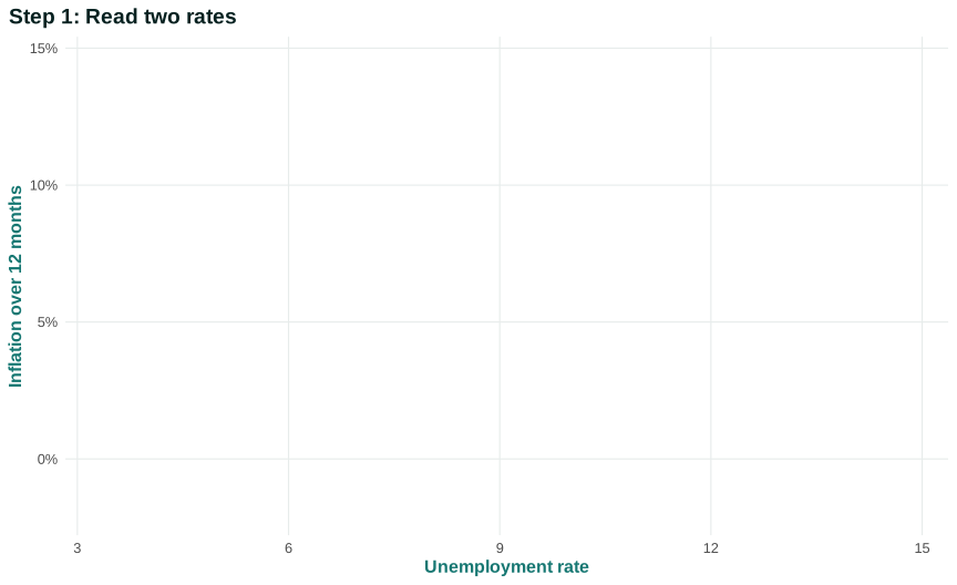
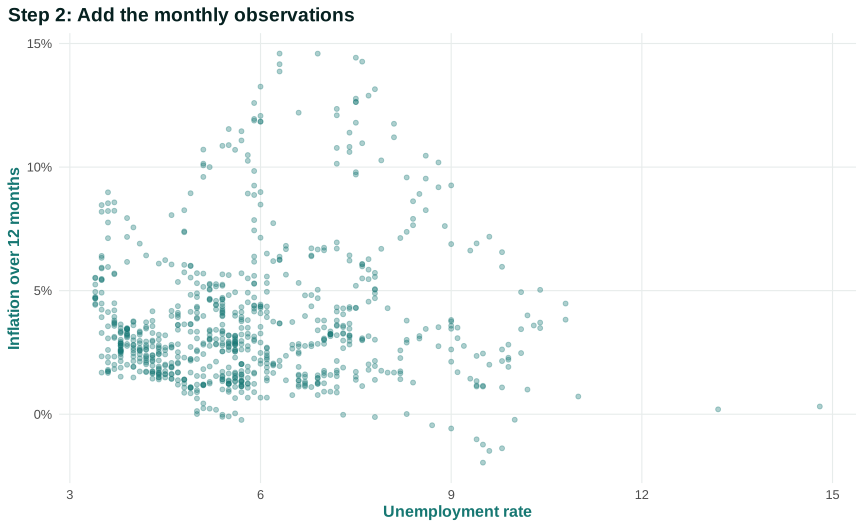
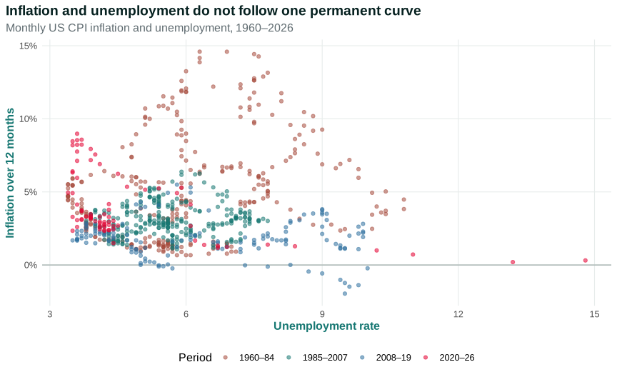
Figure 8.1 plots monthly US unemployment on the horizontal axis and twelve-month CPI inflation on the vertical axis. Each point is one month. The final step colors broad periods. These colors are descriptive groupings, not estimates of stable regimes or causal breaks.

Step 1: Read two rates

Blank inflation and unemployment axes.

Step 2: Add monthly observations

Monthly US inflation and unemployment observations.

Summary figure

Figure 8.1: Monthly US CPI inflation and unemployment by broad period, 1960–2026. Source: BLS via FRED.

Open the live step-by-step figure

First read one point. A point near 4 on the horizontal axis and 3 on the vertical axis represents a month with about 4 percent unemployment and 3 percent inflation from twelve months earlier. It does not represent the inflation that occurred within that single month. Nor does it say unemployment caused inflation.

Now compare the colored clouds. The 1960–84 observations include high-inflation combinations that are largely absent from 1985–2007. The 2008–19 period contains many low-inflation observations despite changing unemployment. The 2020–26 points include an unusual pandemic unemployment spike and a later inflation surge. One permanent fitted line would compress these differences and obscure changed supply conditions, expectations, institutions, and policy.

The plot also suppresses time order within each color. A month in the lower right may be followed by a month in the upper left, but the scatterplot does not show the path. Inflation is measured over twelve months while unemployment is a current monthly rate, so their windows do not align perfectly. Wage bargaining, production, and policy operate with lags. A looped path through the scatter can look like a weak cloud even when a time-sequenced mechanism is operating.

Aggregation hides sectors. Unemployment can be high in hospitality and low in logistics; price increases can begin in vehicles and later move to rents. National monthly points combine regions, industries, workers, and contracts. Disaggregation does not automatically solve causal identification, but it tells us where a mechanism should appear first.

The vertical axis is CPI inflation, while some policy analysis uses PCE inflation. Chapter 7 explained why the measures differ in scope, weights, formula, and revision. A relationship estimated with one inflation measure need not be numerically identical with another. The theoretical question is not “Which scatterplot is true?” but “Which measure and slack concept match the mechanism being tested?”

The Phillips curve is a relationship between inflation and economic slack under stated conditions. It can organize evidence and model mechanisms. It is not a permanent menu from which policymakers select any unemployment–inflation combination. The figure does not reveal lags, expectations, supply shocks, bargaining institutions, or which direction causation runs. TE 2.0 inflation mechanism sequence

Our central question therefore requires mechanisms: How can demand, supply, expectations, and distributional conflict produce inflation? We will introduce actors and decisions before using labels. We begin with one demand-pressure chain, then change the initiating condition to a supply shock, and finally examine how contracts, expectations, power, and policy shape persistence.

Questions

Review the live step-by-step figure

Question 8.1. What is the strongest conclusion from Figure 8.1?

1. One permanent Phillips curve fits every decade
2. The inflation-unemployment relationship changes across periods
3. Unemployment causes every price change
4. Supply shocks never matter

Exercise

A shifting relationship

Use Figure 8.1 to explain why fitting one permanent inflation-unemployment line would be misleading.

The model solution is available in the restricted instructor materials.

8.2 Demand pressure and bargaining

Imagine that households, firms, government, or foreign buyers increase planned spending on US production. Firms receive more orders and see inventories decline relative to plans. Some increase production and post vacancies. The first response is not necessarily a price increase: firms can use idle capacity, add hours, hire workers, change delivery times, accept a smaller margin, or raise prices.

The labor-market response depends on conditions built in Chapters 2–4. When vacancies rise and unemployment is low, workers may find alternative jobs more easily. A worker who can credibly leave has a stronger outside option. Firms trying to recruit, retain, and motivate workers may need to offer faster nominal-wage growth. Collective bargaining, minimum wages, immigration status, discrimination, occupational licensing, scheduling authority, and unemployment insurance can change the response.

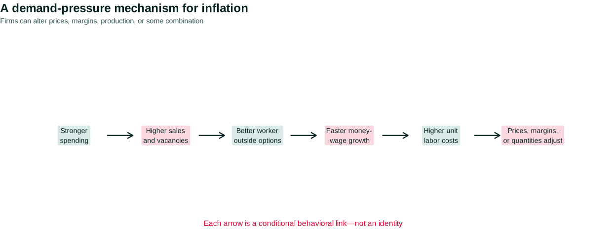
Money-wage growth becomes a cost pressure when it exceeds labor-productivity growth, other things held fixed. Unit labor cost is labor compensation per unit of output. If compensation per hour rises 5 percent and output per hour rises 2 percent, unit labor cost rises by roughly 3 percent. That arithmetic does not dictate a 3 percent price increase. Firms can alter margins, technology, product quality, quantities, or prices.

Use a small numerical example. A firm initially pays $30 in labor compensation for each unit it produces and sells the unit for $50. Other unit costs are $10, leaving a $10 margin before fixed costs and other claims. Now labor compensation per unit rises to $31.50. If the selling price remains $50 and other costs remain $10, the unit margin falls to $8.50. The firm can accept the smaller margin, raise price to $51.50 to restore it, reduce other costs, improve productivity, or change output. The accounting identifies feasible combinations; behavior and market conditions determine the choice.

Situation	Labor cost per unit	Other unit cost	Selling price	Unit margin
Initial	$30.00	$10.00	$50.00	$10.00
Absorb labor-cost increase	$31.50	$10.00	$50.00	$8.50
Restore prior dollar margin	$31.50	$10.00	$51.50	$10.00

The table also separates a dollar margin from a markup rate. Restoring a $10 dollar margin after costs rise does not keep every percentage ratio unchanged. A firm may target a margin over costs, a return on assets, a market share, cash flow, or survival. Treating “the firm” as mechanically applying one markup erases strategy, finance, and competition.

Productivity changes the link from wages to unit costs. If compensation per hour rises 5 percent while output per hour also rises 5 percent, labor compensation per unit is approximately unchanged. Productivity can increase through technology, training, reorganization, or more intense work, and those channels have different effects on workers. An employer can raise measured output per hour while shifting risk or worsening working conditions. A macro cost calculation does not settle welfare.

Time matters too. Firms may initially meet demand from inventories and change prices later. Workers may change jobs before annual wage reviews. Posted prices can adjust faster than wages, or vice versa. A cross-sectional correlation between current wage growth and current inflation may miss these lags and can reflect common demand or supply causes.

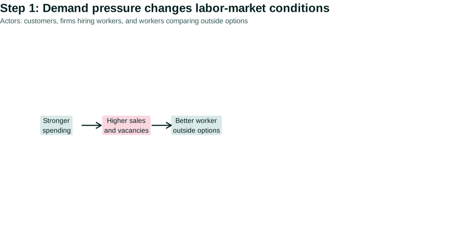
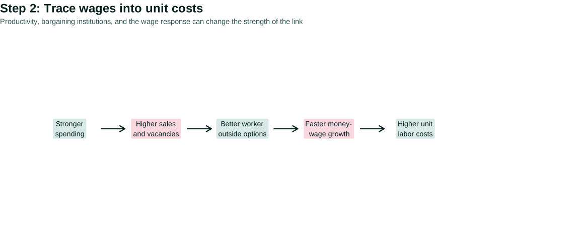
Figure 8.2 stages this chain. It is an analytical figure, not a claim that every historical inflation episode traveled through all six boxes with the same strength.

Step 1: Spending, vacancies, and outside options

The first three links in a demand-pressure chain.

Step 2: Add wages and unit costs

Demand pressure traced into wage growth and unit labor costs.

Summary figure

Figure 8.2: A conditional demand-pressure mechanism for inflation.

Open the live step-by-step figure

Read the arrows as questions. Did stronger spending raise sales or mostly imports? Did firms have unused capacity? Did vacancies improve workers’ outside options across the labor market or only in selected occupations? Did nominal wages respond? Did productivity change? Did firms pass higher unit costs into prices, reduce margins, or cut production? Each arrow requires evidence.

Market power affects the final link. A firm facing little competition may be more able to raise its markup when demand is strong. Another firm may raise prices only enough to prevent its existing margin from shrinking. Aggregate profit growth is not by itself proof of a markup cause: profits can rise because output, sector composition, asset values, or other revenues change. A causal claim needs an appropriate denominator, timing, comparison group, and mechanism.

The sequence is often called demand-pull inflation, but the label should follow the mechanism. It does not mean workers uniquely cause inflation. Spending decisions, employer hiring, worker bargaining, productivity, market power, imports, and policy all enter the chain. Strong demand can also raise output and employment before capacity constraints become important.

Distribution enters immediately. Higher employment can benefit workers who would otherwise be jobless. Faster wage growth can improve purchasing power if it outpaces relevant prices. Price increases can protect or expand profits. Monetary restraint later used to slow demand can operate through housing, credit, investment, and unemployment. A complete account identifies both the inflation mechanism and who gains or bears risk during adjustment.

Demand pressure is one initiating condition. Now change it. Suppose the economy loses access to an important input even though spending has not risen.

Questions

Question 8.2. In a demand-pressure mechanism, lower unemployment can…

1. strengthen worker outside options and wage growth
2. automatically lower every wage
3. eliminate capacity limits
4. prove workers caused inflation

Exercise

Demand mechanism

Trace strong demand through vacancies, outside options, wages, unit costs, prices, and margins; identify one ambiguous link.

The model solution is available in the restricted instructor materials.

8.3 Supply shocks and relative prices

A supply shock changes production costs or productive capacity at a given level of aggregate demand. An oil disruption makes transport and energy-intensive production more costly. A crop failure reduces food availability. A pandemic can make face-to-face production unsafe and close particular workplaces. A damaged port or missing semiconductor can constrain multiple downstream industries.

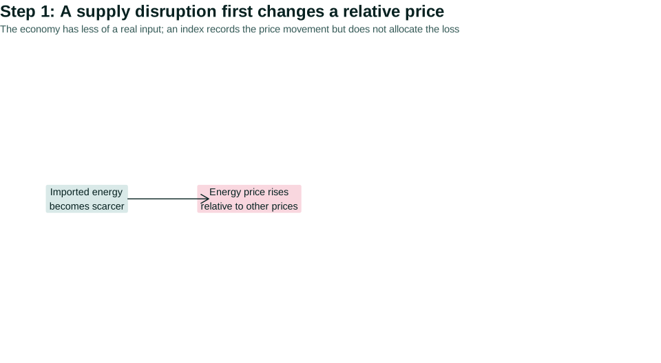
Start with real resources. If imported energy becomes scarcer, the economy must give up more exports or other purchasing power to obtain it, use less energy, or reorganize production. The price increase signals scarcity and allocates demand, but it does not restore the missing resource. Real national income available to domestic groups can fall.

A numerical table makes the real loss visible. Suppose the economy initially produces 100 units of domestic output and trades 5 of them for imported energy. Domestic residents retain 95 units. After the foreign energy price doubles, obtaining the same energy would require 10 domestic units, leaving 90. Alternatively, the economy can import less energy and change production. Either way, there is no purely nominal policy that recreates the missing purchasing power.

Situation	Domestic output	Domestic output transferred for energy	Domestic output remaining
Before the shock	100	5	95
Same energy quantity at higher foreign price	100	10	90

This terms-of-trade example is deliberately simple. Exchange rates, foreign demand, inventories, domestic energy production, and substitution can alter the result. Its purpose is to show why the loss cannot be eliminated by having every domestic group raise its nominal income. The nominal claims can rise together while available real goods do not.

An energy-price increase is initially a relative-price change: energy becomes more expensive compared with other goods. The measured price level rises because energy has weight in the basket and enters other production costs. Continuing inflation requires repeated increases across periods. The first price change can fade from the twelve-month calculation unless it propagates.

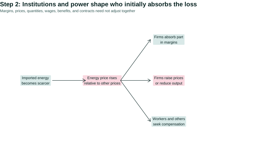
Figure 8.3 separates the initial shock from propagation. The first step shows scarcer imported energy and its relative price. The second step identifies several ways the real loss may initially be absorbed. The final step asks whether repeated adjustments broaden inflation.

Step 1: Change a relative price

Scarcer imported energy raises its relative price.

Step 2: Trace who absorbs the loss

Margins, prices, quantities, and compensation as alternative adjustment paths.

Summary figure

Figure 8.3: Conditional propagation from a supply shock to broader inflation.

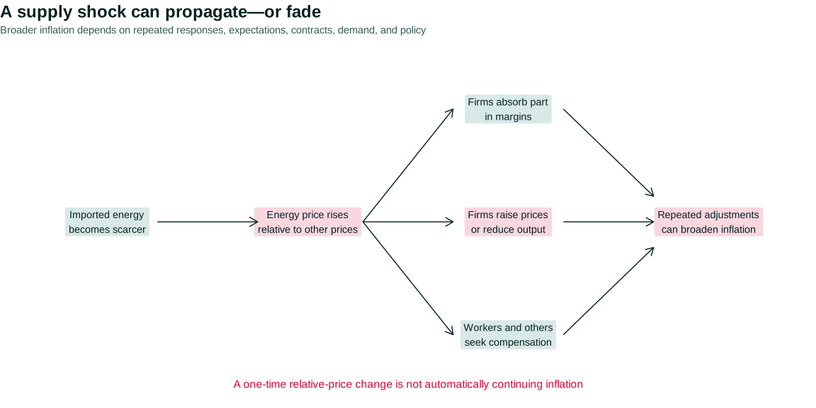
Open the live step-by-step figure

Suppose a restaurant’s energy and ingredient costs rise. The owner can accept a smaller margin, raise menu prices, reduce portions, change inputs, cut hours, or close. Workers can seek wage increases to protect purchasing power. Customers can substitute, reduce restaurant purchases, or accept higher prices. Government can change taxes, transfers, regulations, or public provision. Creditors and landlords can enforce or renegotiate nominal claims. Authority and outside options shape which choices are feasible.

Pass-through describes how much an input-cost or exchange-rate change appears in downstream prices. It is not a fixed coefficient for all firms. Pass-through can be higher when demand is strong, inventories are low, contracts reset quickly, and customers have few substitutes. It can be lower when competition is intense, firms expect the shock to reverse, customers are price-sensitive, or margins were initially high. The same oil-price shock can therefore produce different inflation across countries and periods.

Quantity rationing is another response. A dealer facing too few cars may keep posted prices stable but have long waiting lists, fewer discounts, and lower sales. A hospital can face staff shortages expressed as delayed care rather than a market-clearing price. Official price indexes capture observed transactions and quality adjustments, but shortages and waiting time can impose welfare costs not fully recorded as inflation.

The Interdependence principle explains propagation. One sector’s selling price is another sector’s cost. A wage is income to a worker and cost to an employer. A firm’s margin funds profit income and investment. A tax or transfer changes public and private budgets. Because the links run in several directions, “cost-push” does not identify one guilty actor.

Quantities help diagnose the initiating condition. A negative supply shock tends to raise a relevant price while reducing the affected quantity, other things equal. Stronger demand tends to raise both price and quantity. But actual data contain multiple shocks and lags. Production can rise in one category while falling elsewhere; inventories and imports can temporarily blur the signal. The diagnosis requires more than a headline price index.

An adverse supply shock also creates a policy trade-off. Restraining demand can reduce second-round pressure but cannot produce missing oil, crops, or semiconductors. Supporting incomes can protect vulnerable households but may sustain spending when supply is constrained. Supply measures can help when they directly relax the bottleneck, but they take time and can create new distributional conflicts. Chapters 9 and 10 will examine fiscal and monetary authority in detail.

The initial shock explains a change in costs and relative prices. To understand why inflation may persist after the shock eases, we next need contracts and expectations.

Questions

Question 8.3. A supply shock is…

1. a change in costs or productive capacity at given demand
2. any increase in household spending
3. always permanent inflation
4. the unemployment definition

Exercise

Relative price or inflation

Explain when an oil-price increase remains a relative-price change and when it propagates into broader inflation.

The model solution is available in the restricted instructor materials.

8.4 Expectations and persistence

Wages and prices are not reset simultaneously. A union contract may last several years. A nonunion employer may review pay annually. A landlord may change rent at lease renewal. A restaurant can reprint a menu quickly; a regulated utility may need approval. Social Security adjusts on a statutory calendar. These differences make chronology part of the mechanism.

Inflation expectations are beliefs about future inflation that can affect current decisions. A worker expecting higher prices may seek a larger nominal raise. A firm expecting higher input costs may adjust prices earlier. A lender expecting inflation may require a higher nominal interest rate. Expectations can be based on recent experience, forecasts, contracts, public communication, or social networks; households, firms, and financial markets need not agree.

Measurement is therefore difficult. A household survey may ask for expected inflation over the next year or several years. Professional forecasters answer with models and institutional knowledge. Financial-market measures combine expected inflation with risk and liquidity compensation. Firms may report expected selling prices or input costs rather than a national price index. These objects should not be substituted without explanation.

Households also interpret the question through salient purchases. Food, gasoline, and rent are frequent and memorable; an official index includes a much broader basket. A respondent can reasonably forecast personal cost growth that differs from CPI or PCE inflation. Variation across respondents is information about unequal experience and uncertainty, not merely error to average away.

Expectations can be backward-looking, forward-looking, or rule-based in different contexts. A landlord may look at nearby rents, a union at past CPI and expected future prices, and a retailer at supplier quotes and competitors. The technical labels “adaptive” and “anchored” are useful only after the updating mechanism has been described.

Figure 8.4 uses a stylized contract calendar. Group A reviews in months 1 and 7, Group B in months 3 and 9, and Group C in months 5 and 11. The offsets mean that a common shock enters different nominal terms over time.

Step 1: One contract calendar

One group reviews its contract twice during a year.

Step 2: Add staggered groups

Three groups review contracts in different months.

Summary figure

Figure 8.4: A staggered contract calendar and inflation persistence.

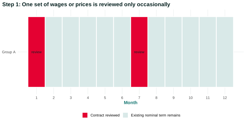
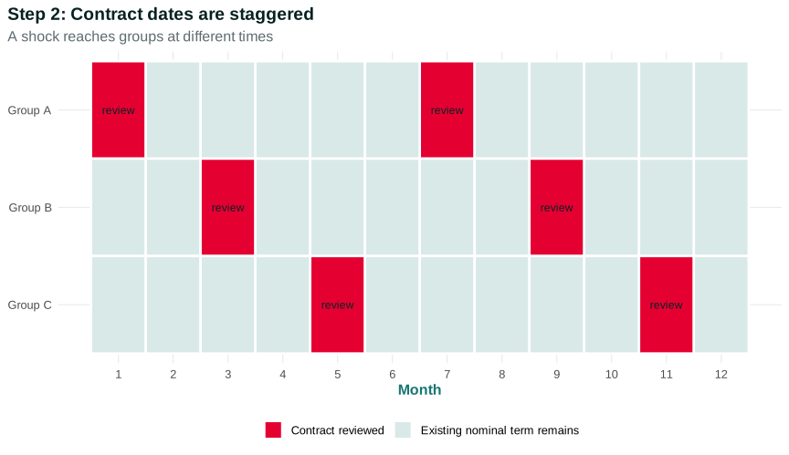
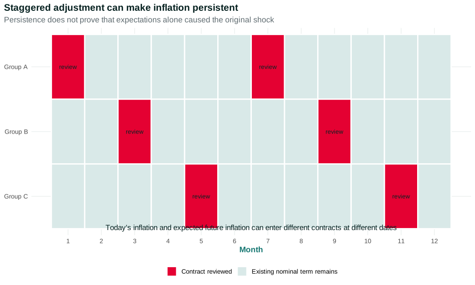
Open the live step-by-step figure

Suppose energy prices jump in month 1. Group A can respond immediately. Groups B and C initially remain under older terms. When their review dates arrive, they observe both the original shock and the price or wage changes made by earlier groups. Their decisions may incorporate expected future inflation. Even if energy stops rising, the sequence can continue while contracts catch up.

Inertial inflation describes persistence produced by staggered contracts, backward-looking rules, and gradual adjustment. It is a mechanism, not a claim that people irrationally repeat the past. A worker seeking to recover lost purchasing power or a firm restoring a prior margin can produce persistence through ordinary goal-directed choices.

Expectations can become more firmly anchored when people believe institutions will keep longer-run inflation near a target. But “anchored” is not a switch that a central bank controls perfectly. Credibility depends on past outcomes, political authority, communication, fiscal conditions, labor-market institutions, and whether policy promises are feasible. Survey expectations, market compensation measures, and forecasts measure different populations and include different risks.

The calendar reveals a causal caution. Observing that expectations rose before some later prices does not prove expectations caused the original episode. Expectations may have responded to supply disruptions, demand, or policy. Conversely, stable long-run expectations do not rule out short-run inflation from relative-price shocks. A good explanation distinguishes initiation from propagation.

Staggered adjustment explains why claims are revised at different dates. We now need to ask whether all groups’ desired real claims can be satisfied simultaneously.

Questions

Question 8.4. Why can expectations affect current inflation?

1. They enter current wages, prices, contracts, and interest rates
2. They determine GDP by identity
3. They erase supply constraints
4. They are always accurate

Exercise

Expectations

Compare backward-looking and anchored expectations after the same one-time supply shock.

The model solution is available in the restricted instructor materials.

8.5 Distributional conflict

Workers seek real wages compatible with living standards. Firm owners seek profits and margins compatible with their plans. Foreign suppliers seek payment for scarce inputs. Landlords, creditors, benefit recipients, and government make claims through rents, debt contracts, transfers, and taxes. Each nominal claim can be individually understandable while the combined real claims are infeasible.

Distributional conflict occurs when groups’ desired real-income claims cannot all be met from available real output. Inflation can be part of the adjustment as groups change nominal wages and prices in attempts to protect their shares. This framework does not require every group to have equal power or responsibility. It directs attention to positions, institutions, and sequence. Wendy Carlin’s distributional-conflict emphasis

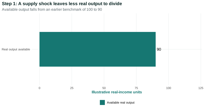
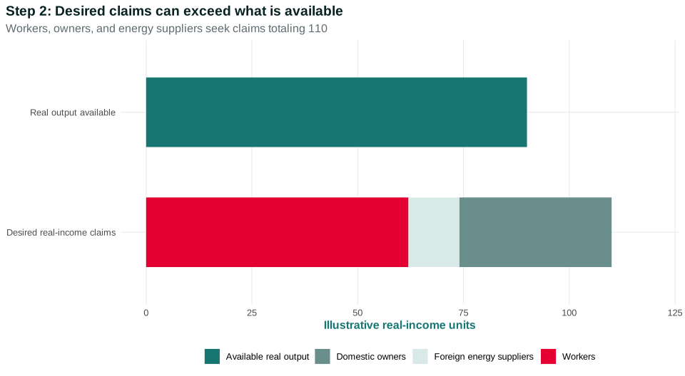
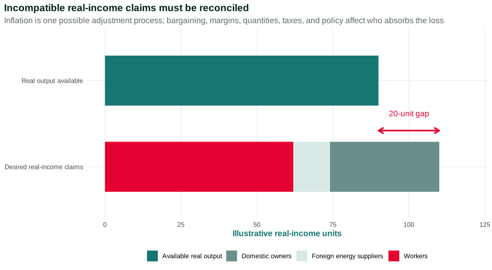
Figure 8.5 uses illustrative units. Before a shock, the economy’s real output benchmark was 100. After an imported-energy shock, only 90 units are available for domestic use. Workers seek 62, domestic owners 36, and foreign energy suppliers 12. Claims total 110. The values are transparent model assumptions, not estimates of US income shares.

Step 1: Available real output

Ninety illustrative units of real output remain after a supply shock.

Step 2: Add desired claims

Desired claims of workers, domestic owners, and foreign suppliers total 110.

Summary figure

Figure 8.5: A twenty-unit gap between available output and desired real-income claims.

Open the live step-by-step figure

The gap is not an accounting error. It is a statement about incompatible plans. Realized claims must eventually fit the 90 units available. Workers may accept lower real wages, owners lower real profits, foreign suppliers fewer purchases, or government lower real services or larger taxes. Output and employment can fall further. Inflation can erode fixed nominal claims. Bargaining and policy determine the path.

Consider three possible adjustment paths. In the first, firms raise prices while nominal wages change slowly, so workers’ real wages fall and profit margins are protected. In the second, strong bargaining produces catch-up wage growth while firms accept smaller margins. In the third, prices and wages both rise repeatedly while monetary and fiscal policy eventually reduce demand and employment. Each path reconciles some claims, but it distributes loss differently.

Adjustment path	First nominal change	Main real-income bearer initially	Possible feedback
Price-led	Output prices rise before wages	Wage-dependent households and fixed-income recipients	Catch-up wage demands and substitution
Wage catch-up	Wages rise after prior prices	Owners if margins compress; customers if prices follow	Further price revision or productivity response
Demand restraint	Interest-sensitive spending and employment fall	Borrowers, workers at risk of job loss, affected firms	Lower sales and wage/price pressure

No row is inevitable. Institutions determine contract timing, price-setting authority, collective bargaining, benefit indexation, credit transmission, and public support. The framework invites empirical questions: Which claim moved first? Which group had a credible outside option? Did margins rise or fall relative to costs? Did output contract? Which nominal contracts remained fixed?

Cooperation can also reduce conflict. Firms and workers might negotiate temporary arrangements, governments can target compensation to those least able to bear the shock, and public investment can relax a supply constraint. Cooperation does not make the real loss disappear, but it can change efficiency, legitimacy, and risk distribution. The Gains from cooperation and conflicts over their distribution principle is visible in both production and adjustment.

Power changes whose nominal claim adjusts first and whose real claim is protected. A large firm with price-setting power may pass costs to customers. A subcontractor may be unable to do so. A union may negotiate catch-up wages; an individual worker may not. A benefit indexed with a lag loses purchasing power temporarily. A creditor with a fixed nominal asset may bear unexpected inflation; a debtor with variable interest may face policy-rate increases.

The framework also clarifies why monocausal blame is misleading. Saying “wages caused inflation” ignores the price and profit claims workers are responding to. Saying “profits caused inflation” can ignore supply losses, demand, sector composition, and wage adjustment. Either claim can become a testable hypothesis only when it specifies authority, timing, counterfactual behavior, and evidence.

Distributional conflict can occur after demand pressure as well as a supply shock. When desired spending exceeds the economy’s capacity, firms, workers, and asset owners may make claims that cannot all be satisfied at current prices and productivity. The distinctive point is not one initial cause. It is that inflation adjusts nominal values while the struggle is over real resources.

The next section compares demand and supply evidence and asks how policy alters the adjustment rather than pretending to eliminate trade-offs.

Questions

Question 8.5. Distributional conflict occurs when…

1. all real-income claims can be satisfied easily
2. workers, firms, and others seek real claims exceeding available output
3. only one price changes once
4. no group has power

Exercise

Inconsistent claims

Construct a numerical example in which desired real wages and profit margins cannot both be maintained after productivity falls.

The model solution is available in the restricted instructor materials.

8.6 Demand shocks, supply shocks, and policy

Policy requires a diagnosis under uncertainty. The same inflation rate can accompany different movements in output, employment, quantities, wages, margins, imports, and expectations. A single headline cannot identify the appropriate instrument.

Evidence	Stronger aggregate demand	Negative supply shock	Why the comparison is not decisive alone
Output and employment	Often rise initially when capacity is available	Often fall in affected sectors	Multiple shocks and policy can offset the movement
Price and quantity in an affected category	Tend to move in the same direction	Tend to move in opposite directions	Inventories, imports, lags, and measurement matter
Vacancies and worker outside options	Often strengthen	Can differ across sectors	A supply shock can coexist with a tight labor market
Unit labor costs	Can rise through wage pressure	Can rise if productivity falls or wages catch up	Unit costs combine wages and productivity
Margins	May rise when demand is strong	May rise or fall depending on pass-through and power	Aggregate profits are not direct markup estimates
Inflation expectations	May respond to persistent pressure	May respond if the shock propagates	Expectations can be effect and cause

A demand expansion can raise output and employment before producing more inflation as constraints tighten. A negative supply shock can raise inflation while reducing output. Monetary restraint lowers demand in either case, but the benefit–cost comparison differs. Against demand pressure, restraint addresses an initiating condition. Against a supply shock, it may prevent propagation while adding an output and employment loss to the original real-resource loss.

Policy timing creates an additional trade-off. Acting quickly may prevent expectations and contracts from adjusting to high inflation, but policymakers observe noisy and revised data. Waiting can reveal whether a shock is temporary, but it can allow propagation. The decision is not between perfect foresight and negligence. It is a choice under uncertainty with asymmetric costs.

Automatic fiscal stabilizers respond without a new vote: taxes fall and transfers rise when income and employment decline. They can cushion a contraction caused by restrictive policy. Discretionary fiscal action can be more targeted but arrives through legislative, administrative, procurement, and implementation lags. A central bank can change its policy rate quickly, but the effects on demand and inflation unfold through contracts and balance sheets over time.

Policy coordination is neither automatic nor always desirable. Fiscal authorities may seek employment, public investment, or redistribution while the central bank restrains demand. State and local governments can cut spending because of balanced-budget rules just as federal stabilizers expand. Financial regulators can change credit conditions. The aggregate outcome reflects several institutions with different mandates and constituencies.

Supply-side responses also vary in horizon. Releasing reserves can temporarily increase a commodity’s availability. Removing a bottleneck, expanding care infrastructure, changing immigration rules, or investing in energy capacity can affect supply with delays and distributional consequences. Looser competition policy is not a short-run inflation instrument, while emergency anti-price-gouging rules can affect allocation and incentives. The chapter’s mechanism test applies: name the actor, constraint, timing, and expected quantity response.

The central bank changes a short-term policy rate, not every borrowing cost or spending decision directly. Banks, bond markets, mortgage lenders, exchange rates, asset prices, firms, and households transmit the change. Borrowers and sectors that depend on refinancing can respond quickly; wealthy households with fixed-rate assets may respond differently. Chapter 10 will unpack this transmission.

Fiscal policy can change aggregate demand, disposable income, public purchases, taxes, and productive capacity. Targeted transfers can protect households facing food or energy costs but can also sustain spending. A broad tax cut and a public investment project have different timing and supply effects. Chapter 9 will distinguish automatic stabilizers, discretionary actions, financing, and debt.

The Rules of the game principle asks who has authority and under what mandate. The Federal Reserve has statutory goals and operational independence within a political system. Congress and the president make tax and spending law. State and local governments face different budget rules. Firms and unions negotiate within labor and competition law. Policy is not chosen by one benevolent actor with complete information.

Every response has incidence. Higher interest rates can slow inflation by reducing interest-sensitive spending, investment, construction, and eventually employment. Fiscal restraint can reduce public services or household income. Supply policy can change environmental costs, property claims, and industry power. An analysis that names only the average inflation effect leaves out who bears adjustment risk.

Use a controlled thought experiment. Begin with inflation above the policy goal, output near capacity, and stable supply conditions. A policy-rate increase raises borrowing costs, lowers some asset prices, strengthens incentives to postpone interest-sensitive spending, and reduces planned investment. Sales and vacancies weaken; wage and price pressure may slow. Now change only one condition: the inflation came from an abrupt imported-energy loss and output was already falling. The same rate increase still reduces demand, but it cannot restore energy and may deepen the output loss. The comparison clarifies why diagnosis matters without claiming policymakers observe shocks perfectly.

Next change the household position. A renter hoping to buy a first home faces higher mortgage rates and may postpone purchase. A homeowner with a fixed-rate mortgage is initially insulated. A bank depositor may receive higher interest; a variable-rate borrower pays more. A construction worker faces employment risk as projects slow. The average demand effect travels through unequal contracts and balance sheets.

Now change the fiscal instrument. A broad transfer raises disposable income for many recipients and may support demand. A targeted energy rebate protects exposed households but can weaken the incentive to conserve unless designed carefully. Public investment in grid capacity or transit may expand future supply but has procurement and construction lags. Spending cuts reduce demand more quickly when they cancel current purchases, yet they also reduce public services and contractor income. “Fiscal policy” is not one homogeneous lever.

Policy credibility should also be unpacked. A central bank announcement matters only insofar as households, firms, and financial intermediaries believe it changes future actions and outcomes. Credibility can reduce the output cost of disinflation in some models by changing expectations, but costly policy follow-through may be required to establish it. Democratic legitimacy and distribution affect whether commitments remain politically sustainable.

We will defer a full policy evaluation to Chapters 9 and 10. Here the conclusion is narrower: shock diagnosis changes the expected output, inflation, and distributional consequences of a policy response. The post-pandemic episode provides a useful test because several mechanisms overlapped.

Questions

Question 8.6. Why is a supply shock difficult for demand policy?

1. It can raise inflation while lowering output
2. It always raises output
3. Interest rates change no behavior
4. Distribution never matters

Exercise

Match policy to shock

Compare an interest-rate response to a demand expansion and an energy supply shock, including distributional effects.

The model solution is available in the restricted instructor materials.

8.7 The post-pandemic inflation test

The 2021–22 inflation surge combined rapid demand shifts, disrupted supply, energy and food shocks, fiscal support, changing labor markets, sectoral margins, and expectations. The mechanisms also changed over time. A story that fits early 2021 may not explain 2022 or the later disinflation.

Chronology helps organize evidence. Pandemic closures sharply reduced some services and redirected spending toward goods. Reopening reversed part of that mix. Supply chains and semiconductor production adjusted slowly. Labor supply, vacancies, and job switching changed. Russia’s invasion of Ukraine affected energy and food markets. Policy support protected income and demand. Later, supply constraints eased, demand composition normalized, and monetary restraint strengthened.

Category evidence is necessary because one aggregate rate can conceal offsetting movements. Used vehicles, gasoline, food, shelter, and other services have different production processes and contract timing. Wage data should be compared with productivity and composition. Profit or margin claims require denominators and sector detail. Expectations data require a defined population and horizon.

International comparison can sharpen the diagnosis. Countries experienced common energy, shipping, and pandemic shocks but differed in fiscal support, labor institutions, energy dependence, exchange rates, and price regulation. Similar timing across countries may support a shared shock; different magnitudes can reveal exposure and policy. It still does not isolate one cause because several national differences move together.

Sector sequence matters. Durable-goods inflation rose early as goods demand increased and production constraints tightened. Later price pressure broadened into some services, including categories with slow-moving rents. Energy and food contributions changed again after geopolitical shocks. An explanation should match these turning points rather than applying one label to the whole interval.

Disinflation also requires explanation. It can reflect repaired supply chains, lower energy-price contributions, normalized demand composition, productivity growth, lower margins, slower wage growth, restrictive policy, anchored expectations, or base effects. Falling inflation does not prove that the last policy action caused the entire decline. The counterfactual remains unobserved.

The evidence package should therefore be organized by predictions rather than slogans. A demand account predicts spending and quantity pressure in affected markets. A supply account predicts constrained quantities or rising input costs. A margin account predicts price changes relative to appropriately measured costs. A wage account predicts compensation relative to productivity and contract timing. An expectations account predicts changes in forward-looking decisions. A policy account predicts transmission through rates, credit, spending, vacancies, and lags.

Sources must also be matched. CPI and PCE category data measure prices with different scopes. National accounts provide aggregate incomes and profits but may not identify markups. Employer surveys, household surveys, and administrative records cover different populations. Narrative evidence about supply disruptions can establish chronology while remaining insufficient for magnitudes. A robust conclusion explains what each source contributes and what it cannot establish.

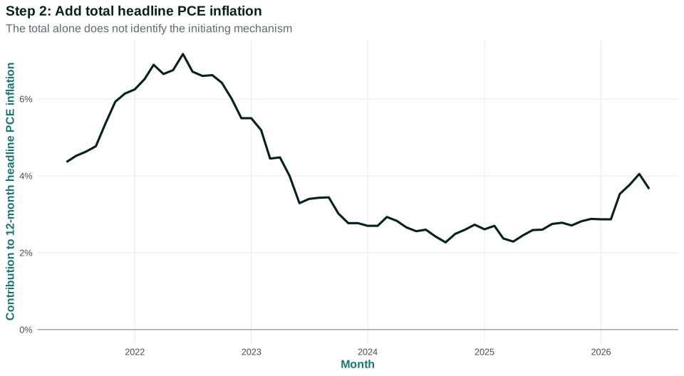
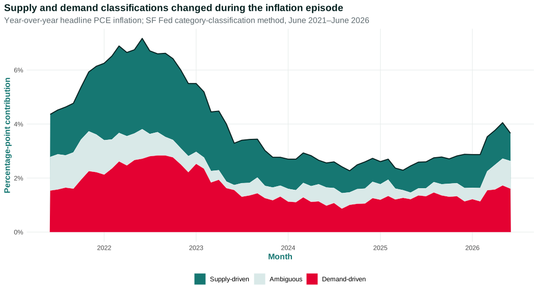
The San Francisco Fed’s supply- and demand-driven PCE data provide one research design. For each PCE category and month, the method estimates unexpected price and quantity changes. If they move in the same direction, the category is classified as demand-driven; if they move in opposite directions, supply-driven; statistically unclear cases are ambiguous. These contributions are then aggregated. SF Fed supply–demand classification

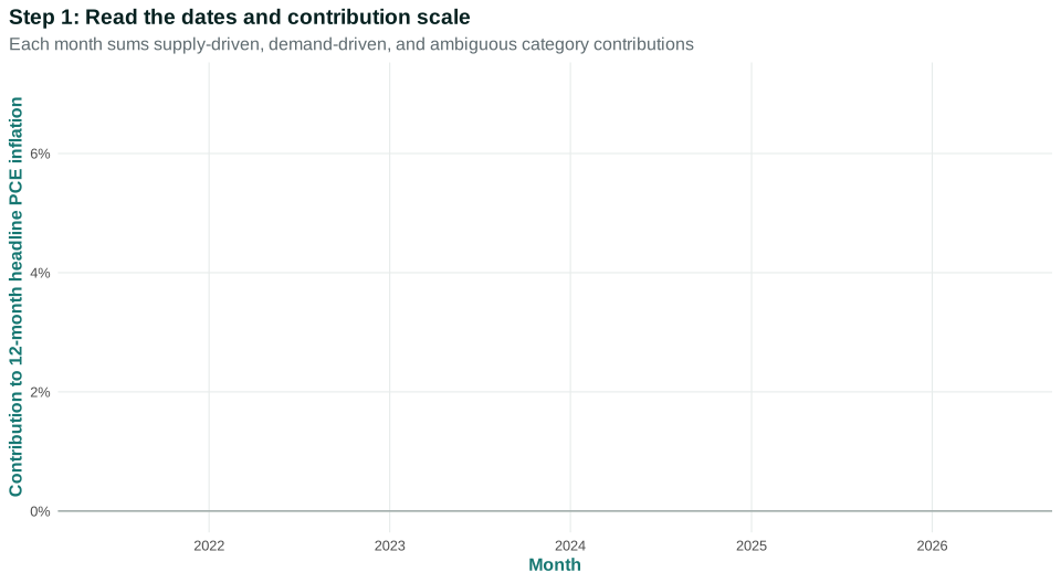
Figure 8.6 uses the published year-over-year headline PCE contributions from June 2021 through June 2026. The line is total headline PCE inflation. The stacked areas show categories classified as supply-driven, demand-driven, or ambiguous in each month.

Data Extension 8.7.1: Supply- and demand-driven PCE inflation

Step 1: Read dates and contribution units

Blank dates and percentage-point contribution axes.

Step 2: Add total headline PCE inflation

Headline PCE inflation calculated from the three published components.

Summary figure

Figure 8.6: Supply-driven, demand-driven, and ambiguous contributions to year-over-year headline PCE inflation. Source: Federal Reserve Bank of San Francisco.

Open the live step-by-step figure

Compare mid-2021, the 2022 high-inflation period, and 2025–26. Both supply- and demand-classified contributions are present, and their importance changes. The ambiguous area is not a nuisance to be discarded; it represents categories for which the method cannot distinguish the sign pattern with sufficient confidence.

The decomposition is evidence against a simple either/or story. It is not direct observation of “true supply” and “true demand.” The classification depends on a model of predicted price and quantity changes, a rolling estimation window, PCE categories, revisions, and statistical thresholds. Another design can produce different shares. A strong interpretation states the method and uncertainty before drawing policy conclusions.

Questions: Which two variables determine whether a category is labeled supply- or demand-driven? Why might a category be ambiguous? Does the presence of demand-driven contributions show that one fiscal program caused the entire inflation episode? What other evidence would be required?

A serious episode diagnosis combines this decomposition with category prices and quantities, wages and productivity, margins with valid denominators, supply-chain measures, expectations, fiscal and monetary timing, and international comparisons. It should state what evidence would falsify its favored explanation.

The post-pandemic episode reinforces the chapter’s central lesson: mechanisms overlap and change. We finish by returning to the shifting relationship in the opening figure.

Questions

Question 8.7. A credible post-pandemic explanation should…

1. match timing and category-level evidence across mechanisms
2. name one cause without comparison
3. treat CPI and PCE as identical
4. use chronology as proof

Exercise

Post-pandemic evidence plan

Design a source register that could distinguish demand, supply, wages, margins, expectations, and policy channels.

The model solution is available in the restricted instructor materials.

8.8 A changing relationship

The opening inflation–unemployment plot did not reveal one permanent curve. We can now say why. Stronger demand can tighten labor and product markets, but bargaining institutions, productivity, margins, and capacity shape transmission. Supply shocks can raise relative prices and reduce real income. Contracts and expectations spread adjustment through time. Distributional conflict affects whose real claim gives way. Policy changes demand, expectations, and risk-bearing—and responds to all of them.

The Principle of aggregation and feedback is central. Wages are costs and incomes. Prices are costs and revenues. Interest payments are expenses to debtors and income to creditors. One firm’s output is another’s input. Expectations respond to outcomes and influence later contracts. The economy is not the sum of independent price decisions.

This does not mean every explanation is equally good. A mechanism should predict timing, category movements, quantities, wages, margins, expectations, output, and employment. It should specify what is held fixed and what would contradict it. A supply account should identify the constrained inputs and quantity evidence. A demand account should identify the spending source and capacity response. A distributional-conflict account should identify claims, institutions, and adjustment sequence.

The Phillips relationship remains useful when its conditions are explicit. It can summarize how inflation responds to slack for given expectations and supply conditions. It becomes misleading when presented as a timeless law or a costless policy menu. “Natural rate,” “NAIRU,” and similar expert labels can hide uncertainty if treated as directly observed constants; detailed stabilization models belong in the next chapters and optional preparation material.

Students preparing for intermediate economics should nevertheless be able to translate the chapter into model language. Demand pressure changes the bargaining gap and firms’ desired price adjustments. A supply shock changes feasible real claims and can move the inflation–slack relationship. Expected inflation affects current wage and price decisions. Policy changes aggregate demand and possibly expectations. The main text teaches these relationships through actors and adjustment; later courses may express them in equations.

Model discipline requires stating the held-fixed conditions. When tracing stronger demand, hold supply conditions and institutions fixed initially. When tracing an energy shock, hold planned demand fixed initially. When examining staggered contracts, hold the initiating shock fixed. After learning each mechanism separately, allow them to interact. Without that staging, a model can “explain” every outcome after the fact and predict none before it.

The chapter also gives a falsification habit. If prices rise while quantities also rise in the relevant categories, a pure negative-supply story needs revision. If wages lag prices and margins rise relative to costs, a wage-first story is incomplete. If long-run expectations remain stable, an expectations-deanchoring account needs more evidence. If policy-sensitive spending does not respond over plausible lags, the claimed transmission channel needs re-examination.

Chapter 9 turns to fiscal policy: automatic stabilizers, discretionary spending and taxes, implementation, budget balances, debt, and incidence. Chapter 10 turns to monetary institutions and transmission: the Federal Reserve, policy rates, credit, asset prices, exchange rates, expectations, employment, and inflation. Neither institution acts outside distributional conflict. Policy changes who spends, who borrows, who works, who receives public services, and who bears risk.

The handoff is therefore institutional as well as theoretical. The models in this chapter identify channels a policymaker may wish to influence, but an instrument is not a channel. Congress cannot instantaneously choose aggregate demand; it legislates taxes, transfers, purchases, and programs implemented by agencies. The Federal Reserve cannot directly choose every wage or price; it changes financial conditions through a banking and market system. The next two chapters will trace those actors, constraints, lags, and distributional consequences with the same mechanism-first discipline used here.

The outcome to remember is not a list of competing inflation labels. It is a method: locate the evidence, identify the actors and real constraint, trace price and quantity responses, add contracts and expectations, ask whose claims are incompatible, and specify what would change the explanation. That method can accommodate plural causes without treating causal judgment as arbitrary.

Seeing the principles in action

Principle	Example	Everyday Economics
Interdependence principle — focal	One sector’s price is another sector’s cost or income, so shocks propagate through supply chains and contracts.	Higher fuel prices affect deliveries, fares, and household budgets.
Doing the best you can principle	Workers, firms, and policymakers adjust wages, prices, and plans given expectations and constraints.	A firm may raise price, accept a smaller margin, or redesign production.
Rules of the game principle — focal	Bargaining systems, indexation, competition, and central-bank mandates shape inflation dynamics.	An indexed contract passes inflation through differently from a fixed contract.
Trade-offs and opportunity costs principle	Restraining demand may reduce inflation but sacrifice output and employment in the adjustment.	Higher interest rates discourage some purchases and investments.
Principle of gains from cooperation and conflict of interest	Production creates gains while distributional conflict concerns real wage, profit, rent, and benefit claims.	After an energy shock, groups contest who absorbs the loss.
Principle of individual and societal interests	Protecting an individual real-income claim can contribute to collectively inconsistent claims.	Every group can seek full compensation even when total real resources fell.
Principle of aggregation and feedback — focal	Wage, price, expectation, demand, and policy adjustments feed back and can amplify or dampen inflation.	Expected inflation can influence today’s contract and tomorrow’s price.

Skills and learning objectives

• Reading a shifting empirical relationship
• Explaining demand and supply inflation mechanisms
• Tracing expectations and persistence
• Analyzing distributional conflict
• Matching policy trade-offs to shocks

Concepts to learn

• Phillips curve
• Demand-pull inflation
• Supply shocks and relative prices
• Inflation expectations and inertia
• Distributional conflict
• Demand versus supply shocks
• Post-pandemic inflation as a multi-causal episode

Glossary

Chapter 8 terms

Phillips curve

A relationship between inflation and economic slack under stated expectations, institutions, and supply conditions.

See also: inflation expectations; supply shock.

demand-pull inflation

Inflation generated when strong aggregate demand presses against productive capacity and influences wages, costs, prices, and margins.

See also: Phillips curve.

supply shock

A change in production costs or productive capacity at a given level of aggregate demand.

See also: Phillips curve.

inflation expectations

Beliefs about future inflation that can affect current wage setting, price setting, contracts, and interest rates.

See also: inertial inflation; Phillips curve.

inertial inflation

Inflation persistence produced by staggered contracts, backward-looking rules, and gradual adjustment of wages and prices.

See also: inflation expectations.

distributional conflict

Conflict among workers, firms, creditors, recipients of benefits, and others over real income claims that cannot all be satisfied at current productivity and output.

See also: inflation expectations.

unit labor cost

Labor compensation required to produce one unit of output, which changes with both compensation per hour and labor productivity.

See also: demand-pull inflation.

Flashcards

Why is the Phillips curve not a permanent menu?

Supply conditions, expectations, institutions, and policy shift the inflation-unemployment relationship.

What turns a relative-price shock into general inflation?

Propagation through costs, wages, margins, contracts, expectations, and policy responses.

What is distributional conflict inflation?

Repeated nominal adjustment when incompatible real-income claims exceed what current productivity and output can sustain.

Questions

Question 8.8. Which can produce disinflation?

1. Weaker demand, easing supply constraints, anchored expectations, or claim adjustment
2. Only falling population
3. Only deflation
4. A higher price level by itself

Exercise

Explain disinflation

Give a multi-causal explanation of falling inflation and state evidence that would falsify it.

The model solution is available in the restricted instructor materials.