Jobs, Output, and Real Wages
Chapter 2 public working draft
Download the current dated PDF snapshot
Public working draft. This is an AI-assisted developmental chapter for coauthor review. Google Docs remains canonical. Source badges identify adapted CORE/UOE material; facts, classifications, exercises, figures, data, rights, and accessibility still require named human review.
Central question: Why can people with similar skills face different jobs and real wages—and why does the wage a firm can feasibly offer depend on employment across the whole economy?
By the end of this chapter, you should be able to: classify labor-market states; distinguish stocks from flows; connect workers, hours, and productivity to output; calculate a real wage; build and interpret a wage-setting curve; distinguish movement along it from a shift; and interpret an empirical wage-setting estimate.
Before adding new ideas, retrieve four measures from Chapter 1.
Chapter 1 retrieval check
- Employment rate: the employed share of the relevant population or labor force, depending on the stated denominator. Always check which denominator is used.
- Unemployment rate: unemployed people as a share of the labor force, not of the entire adult population.
- Real wage: a nominal wage adjusted for a price index so that it describes purchasing power.
- Labor productivity: output per hour worked.
These measures describe different things. None by itself explains why a person finds a job, why a firm offers a particular wage, or why an economy produces a particular level of output. This chapter first sharpens the measurements, then builds one behavioral relationship that helps explain wage offers. It will keep four kinds of statement separate: an accounting identity that must hold by definition; a behavioral relationship about choices; a causal claim supported by a research design; and an aggregation feedback through which conditions across the economy alter individual choices.
2.1 Graduating into a recession
Imagine two students with the same major, similar grades, and comparable work experience. One graduates when firms are expanding; the other graduates when firms are canceling vacancies. Their qualifications matter, but they do not act alone. Each graduate’s outcome also depends on employers’ hiring plans, other applicants, customers’ spending, credit conditions, and expectations about the future. This is the Interdependence principle: the opportunities facing one person depend partly on the choices and circumstances of others.
A recession can change the opportunity set before a graduate makes any choice. Applications may receive fewer replies; acceptable offers may arrive later; a graduate may take temporary work, continue studying, move home, or leave the labor force. Those changes can affect current earnings, later experience, bargaining power, and expectations.
Reading recession-entry evidence one step at a time
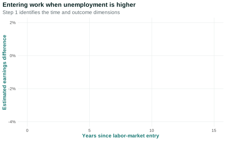
Moving right means following an entry cohort further into its working life. A value below zero on the vertical axis means lower estimated earnings for entrants who began work when state unemployment was higher.
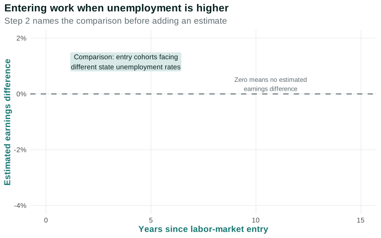
The comparison is across entry cohorts facing different labor-market conditions, not simply the national economy before and after a recession.
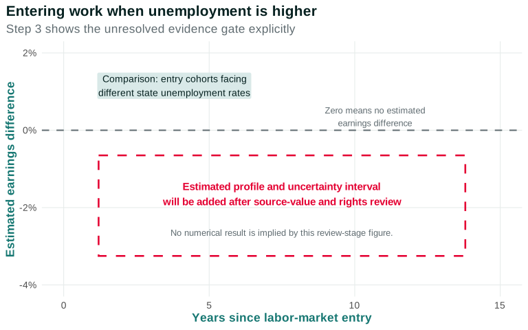
The approved hook will show estimated earnings effects of entering the US labor market when state unemployment is higher, using Hannes Schwandt and Till von Wachter’s “Unlucky Cohorts” study. The current live figure deliberately shows only the reading structure. It does not invent values or reproduce published artwork while the source values, uncertainty, methods, and rights decision remain under review. Source plan
The study follows US labor-market entry cohorts from 1976 to 2015. Its comparison is not simply “graduates in a recession versus graduates in a boom.” The researchers use differences in labor-market conditions across entry cohorts, states, education groups, gender, and race. In the proposed figure, the horizontal axis records age or time since entry. The vertical axis records the estimated difference in earnings associated with a one-percentage-point higher state unemployment rate at entry. A value below zero means that entrants facing the weaker labor market are estimated to earn less at that age, after the study’s specified comparisons and controls.
Step 2: Follow the estimate through time
The memorable pattern is persistence. Earnings and wages are lower for cohorts that enter when unemployment is higher, and the losses do not disappear immediately when a recession ends. The paper also finds larger and more persistent losses among less-advantaged entrants. This does not mean that every person in a cohort loses the same amount. Some find secure jobs quickly, some continue in education, some move, and some have family wealth or professional networks that make waiting less costly. Others accept work that pays less, offers fewer hours, provides less training, or starts on a weaker career ladder.
Step 3: Separate the evidence from the mechanism
The estimate is stronger evidence than a simple national time series because it compares entry conditions across cohorts and places. Even so, one figure cannot reveal every pathway. A weak labor market can affect the number of vacancies, the kinds of firms hiring, the offers workers can afford to reject, early work experience, later job changes, and household decisions. The study tests and discusses several threats to the comparison, including migration and the timing of entry, but the mechanism still requires economic reasoning.
Our task is therefore not to read a complete explanation from the line. It is to explain why the same qualifications can meet different opportunities, why job loss can be more or less costly, and why firms’ feasible wage offers change when employment conditions change across the economy.
Everyday Economics 2.1
The same résumé in a different year
Ask someone who entered work in 2009 or 2020 how many applications they sent, what kind of first job they accepted, and which plans they postponed. Which part of the story was personal choice, and which part reflected the macroeconomy?
The story generates a hypothesis; the cohort study supplies a research design. Evaluating the causal result still requires attention to migration, further study, occupation, family resources, how labor-market entry is dated, and how recovery differs across groups.
Fact-check flag: Verify the Schwandt–von Wachter sample, research design, outcome definitions, and heterogeneity claims against the published paper; add one accessible first-person account. The descriptive unemployment-duration series in Section 2.2 remains separate from claims about long-run scarring.
Questions
Question 2.1. What does the recession-entry study add to the opening story?
- It proves that every graduate experiences the same earnings loss
- It compares otherwise similar entry cohorts facing different labor-market conditions across places and years
- It shows that unemployment duration is the only mechanism
- It reports only the national unemployment rate over time
Exercise
Same résumé different year
Write two paragraphs comparing a person entering work in a strong labor market with a similar person entering in a weak one. In the first paragraph, describe choices and constraints without claiming a cause. In the second, identify one causal question and the additional evidence needed to answer it.
The model solution is available in the restricted instructor materials.
2.2 Labor-market states are stocks connected by flows
Official labor statistics first classify people’s situations. A person is employed if they did paid work during the reference period or had a job from which they were temporarily absent under the survey rules. A person is unemployed if they had no job, were available, and actively sought work, or met the qualifying temporary-layoff rule. Everyone else is outside the labor force. The labor force is employed plus unemployed people. TE 2.0 §1.3
These categories distinguish situations that everyday language blurs. Someone who wants a job but has not searched recently may be outside the labor force. Someone working one paid hour can be employed even if they want full-time work. A caregiver and a retired person may share a statistical category while facing very different choices and constraints.
The number employed in a month is a stock: a quantity measured at a point in time. Hiring, separation, entry, and exit are flows: quantities measured over an interval. Employment can end a month unchanged even when millions of people moved into and out of jobs. TE 2.0 §1.6
Reading the stock-and-flow figure one step at a time
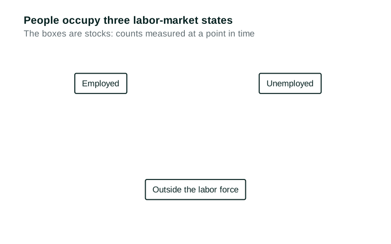
The boxes are mutually exclusive states in this simplified map. The labor force consists of the employed and unemployed boxes.
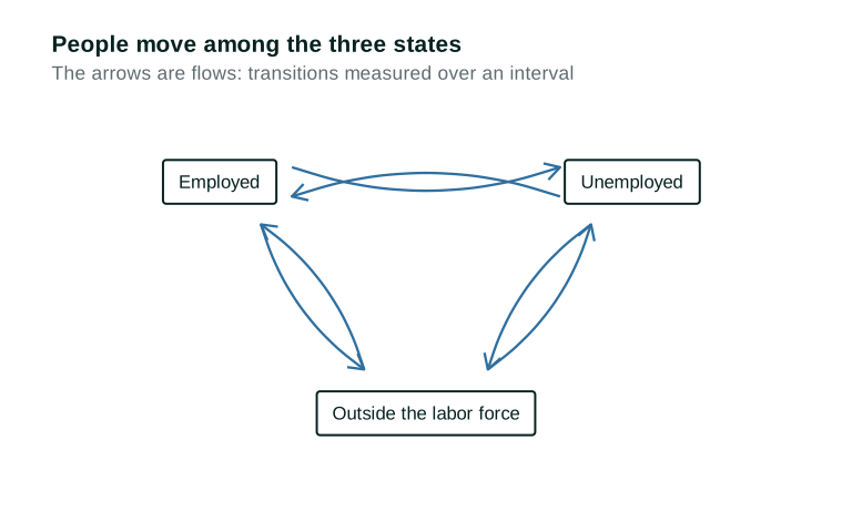
The arrows add movements a snapshot hides: job finding, separation, entry, exit, retirement, and return.
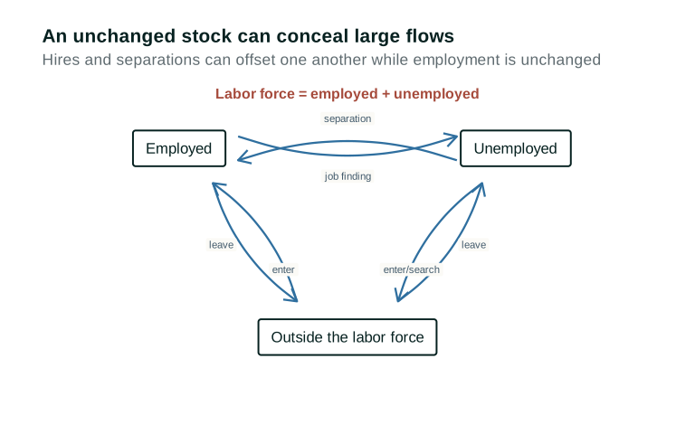
The figure is an accounting map, not a behavioral model. It shows which flows change each stock, but it does not yet explain why those flows change.
Note for fact checkers: Validate the classification language against current BLS CPS definitions, especially temporary layoff, active search, and reference-period wording.
Duration adds information that the unemployment rate alone does not show
The unemployment rate is a stock measure: it tells us the share of the labor force currently unemployed. It does not tell us whether the same people remain unemployed month after month. Two economies could have the same unemployment rate even if one has frequent short spells and the other has fewer but much longer spells.
The next figure reports median weeks unemployed among people who are unemployed in each month’s survey. The median is the midpoint: half report a longer ongoing spell and half report a shorter one. BLS emphasizes two limitations. First, these are spells still in progress, not completed spells. Second, the series does not report how long it takes a person to find a job. People with long spells remain in the measured unemployed population for more survey months, while people who find jobs quickly leave it. BLS/FRED duration evidence
Reading the duration evidence one step at a time
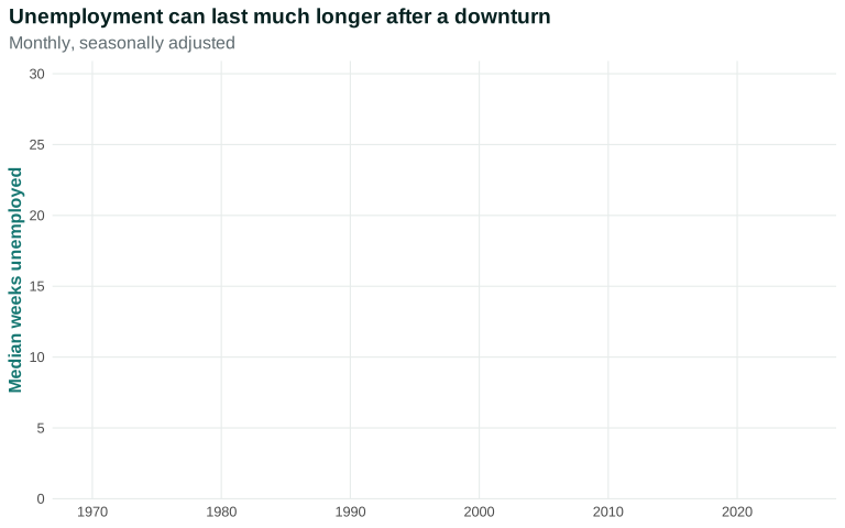
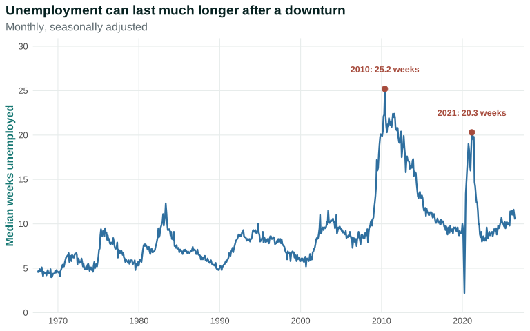
Moving right means moving forward in time. Moving up means that the median person who is currently unemployed reports a longer ongoing spell. The figure is national and covers unemployed people generally; it is not specific to labor-market entrants.
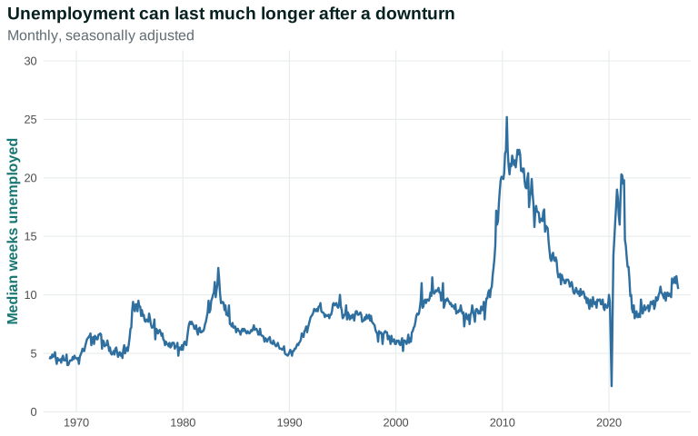
The line rises sharply after some downturns and can remain high after the unemployment rate has begun to fall. That pattern could reflect slow job finding, differences in who remains unemployed, or both. The line does not distinguish those explanations.
Suppose 1,000 people are unemployed at the beginning of a month. If 400 find jobs and 400 newly lose jobs, the unemployed stock can end near 1,000 even though many people moved. If only 100 find jobs while separations remain high, unemployment and average duration can rise together. The stock-and-flow map tells us where the changes occur; a behavioral model is needed to explain why job finding and separation change.
Risk is unequally distributed. Savings, family resources, access to credit, unemployment insurance, health coverage, disability access, citizenship status, discrimination, and local job availability affect how long a person can search and which offer they can reject. These conditions do not change the statistical definition of unemployment, but they change what an unemployment spell costs.
Questions
Review the live step-by-step figure
Question 2.2. Employment begins and ends the month at 160 million. What follows?
- No one was hired or separated
- Net employment change was zero, but gross flows may have been large
- Unemployment must also be unchanged
- Everyone kept the same status
Exercise
Stocks and flows
Classify five people as employed, unemployed, or outside the labor force. Then construct two sets of monthly flows that leave the number employed unchanged and explain what the stock conceals.
The model solution is available in the restricted instructor materials.
2.3 Work, hours, productivity, and output
Aggregate output connects people at work to what the economy produces. In a simple decomposition:
\[\text{output}=\text{workers}\times\frac{\text{hours}}{\text{worker}}\times\frac{\text{output}}{\text{hour}}\]
The final term is labor productivity. Output can change because more people work, average hours change, or output per hour changes. TE 2.0 §1.5
Suppose 100 workers each work 35 hours and produce 50 dollars of output per hour. Total output is $175,000. If employment falls while productivity rises, the direction of output depends on the size of both changes. This is the Principle of aggregation and feedback: individual and firm-level choices add up, and aggregate outcomes feed back into the choices people face.
The equation is an identity: it must hold when the quantities are measured consistently. It does not say that increasing hours causes productivity to stay fixed, or that hiring one more worker mechanically creates demand for the output. Behavioral and causal claims require a mechanism beyond the accounting.
Everyday Economics 2.2
More output without more workers
A restaurant can serve more meals by adding workers, extending shifts, reorganizing the kitchen, or adopting better equipment. Which margin changes workers’ time, and which changes output per hour?
Use a table before the identity
| Workers | Average hours per worker | Output per hour | Total output |
|---|---|---|---|
| 100 | 35 | $50 | $175,000 |
| 90 | 35 | $52 | $163,800 |
| 100 | 34 | $52 | $176,800 |
| 105 | 34 | $52 | $185,640 |
Read across the first row. One hundred workers each supply 35 hours, creating 3,500 hours of work. At $50 of output per hour, total output is $175,000. In the second row, productivity rises but employment falls. Output falls because the loss of 350 hours is larger than the gain in output per hour. In the third row, employment returns to 100 and productivity remains higher, more than offsetting the shorter workweek. The table prevents us from treating “productivity rose” as a complete explanation of output.
Now read the identity as three margins, not three competing stories. Firms can change the number of workers, scheduled hours, and the organization or equipment that affects output per hour. Workers can accept, refuse, or seek different hours, but their choices are constrained by contracts, household responsibilities, transportation, health, and employers’ authority over scheduling. A national total aggregates these decisions across jobs that differ greatly in hours, security, and productivity.
An identity is not a policy prediction
Because workers × hours per worker × output per hour must equal output when the measures are consistent, the identity is useful for checking arithmetic. It does not tell us what happens after one term changes. If a restaurant reorganizes its kitchen, it may serve more meals with the same staff. It may also cut hours, lower prices, attract more customers, or hire additional workers. Which response occurs is a behavioral and causal question.
Composition also matters. Average productivity can rise when low-productivity establishments close, even if no surviving workplace improves. It can fall when many new workers enter jobs where they are still learning. Neither change automatically tells us whether individual workers became more capable or whether living standards improved.
Questions
Question 2.3. Which expression decomposes total output using labor input?
- Workers + hours + output per hour
- Workers × average hours per worker × output per hour
- Output per worker ÷ employment
- Nominal wage × price index
Exercise
Decomposing output
An economy has 100 workers, 35 hours per worker, and 50 units of output per hour. Calculate output. Recalculate after employment falls 5%, hours fall 2%, and productivity rises 3%, and identify each contribution.
The model solution is available in the restricted instructor materials.
2.4 Nominal wages, real wages, and job quality
A nominal wage is measured in current dollars. A price index summarizes the prices of a specified basket relative to a base period. A real wage adjusts the nominal wage for prices so that it tracks purchasing power rather than dollars alone. TE 2.0 §1.4
Suppose the hourly wage rises from $20 to $21, a 5% nominal increase. If the price index rises from 120 to 129, prices rise 7.5%. The real wage falls: $20/1.20 is about 16.67 base-period dollars, while $21/1.29 is about 16.28.
For small changes, a useful approximation is:
\[\text{real-wage growth}\approx\text{nominal-wage growth}-\text{inflation}\]
This calculation still leaves things out. A national price index may not match a household’s purchases. Taxes, benefits, hours, predictability, risk, and working conditions matter. The Trade-offs and opportunity costs principle reminds us that a worker evaluates the whole job against the next-best alternative—not the hourly wage in isolation.
Purchasing power depends on the comparison
A real wage is always constructed with a price index. If the index represents consumer prices, the result asks how much of a consumer basket the wage can buy. A firm comparing labor cost with output may instead use the price of its product or a broader output price index. These are not interchangeable questions. The chapter uses consumer purchasing power when discussing a worker’s living standard and will state the price measure whenever a numerical comparison is made.
The approximation “nominal-wage growth minus inflation” is useful for small percentage changes. It becomes less accurate when changes are large. The level calculation using the price index is the dependable method. Students should also distinguish an hourly real wage from annual real earnings. Annual earnings depend on hours, weeks worked, unemployment spells, and access to paid leave as well as the hourly rate.
A job is a bundle
Consider two offers. Job A pays $22 an hour for a predictable 35-hour week, includes health insurance, and gives schedules two weeks in advance. Job B pays $24 an hour but guarantees only 20 hours, changes schedules with one day’s notice, and provides no paid leave. The higher hourly wage does not make Job B unambiguously better. A worker’s evaluation depends on expected hours, benefits, commuting costs, care responsibilities, safety, autonomy, advancement, and the risk of losing the job.
This is where economic position and power enter the mechanism. A worker with savings, portable health coverage, secure immigration status, accessible transportation, and another credible offer can reject a poor job more easily. A worker who depends on the current employer for income, health coverage, scheduling accommodations, or legal status may face a far more costly refusal. Education can affect available jobs, but it is not a complete measure of class position or bargaining power. Ownership, wealth, authority, collective organization, race, gender, disability, place, and citizenship can shape the feasible set of choices.
Questions
Question 2.4. A nominal wage rises 4% while prices rise 6%. What happens approximately to the real wage?
- It rises 10%
- It rises 2%
- It falls about 2%
- It is unchanged
Exercise
Nominal and real pay
A worker’s hourly wage rises from $20 to $21 while a price index rises from 120 to 129. Calculate the percentage change in nominal pay and the approximate and exact change in real pay. Name one dimension of job quality the result omits.
The model solution is available in the restricted instructor materials.
2.5 From feasible wage offers to wage setting
Now we move from measurement to mechanism. A firm must recruit suitable workers and make it worthwhile for them to stay. Workers compare the entire job with their next-best available alternative. The firm compares wage cost with the effective work, continuity, and cooperation it expects the employment relationship to provide.
Recruitment is only the beginning. Retention, turnover, judgment, cooperation, and effort also matter, and they cannot all be specified and enforced in advance. A firm may therefore find that paying more than the lowest acceptable wage reduces the cost of turnover or supports more reliable effective work. TE 2.0 Figures 1.18–1.20
This language is deliberately about feasible offers, not a wage firms freely choose without constraints. At a given employment level, the firm’s lowest feasible wage must be high enough to attract the desired workers and make job loss costly enough to support effort. A still higher wage may be possible but more expensive; a lower one may fail to recruit, retain, or motivate the workforce the firm needs.
When unemployment is high, another job may take longer to find, so job loss is costly. When employment is high and unemployment low, outside options improve and other firms compete more intensely for workers. A firm must generally offer more to create the same reason to keep the job. Aggregating these feasible firm choices gives the wage-setting curve.
Reading the wage-setting figure one step at a time
Moving right means a larger share of the labor force is employed and unemployment is lower. Moving up means a higher real wage.
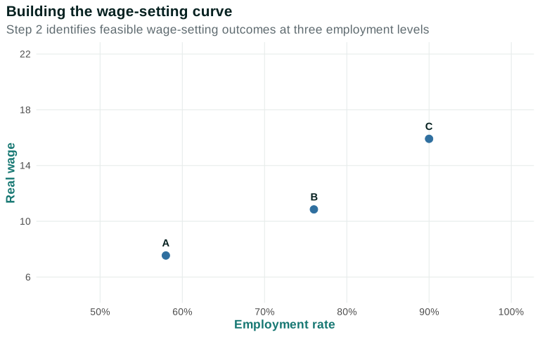
Point A is feasible when employment is relatively low. At B, employment is higher and firms need to offer more. At C, employment is close to the labor-force endpoint and the feasible wage is higher still.
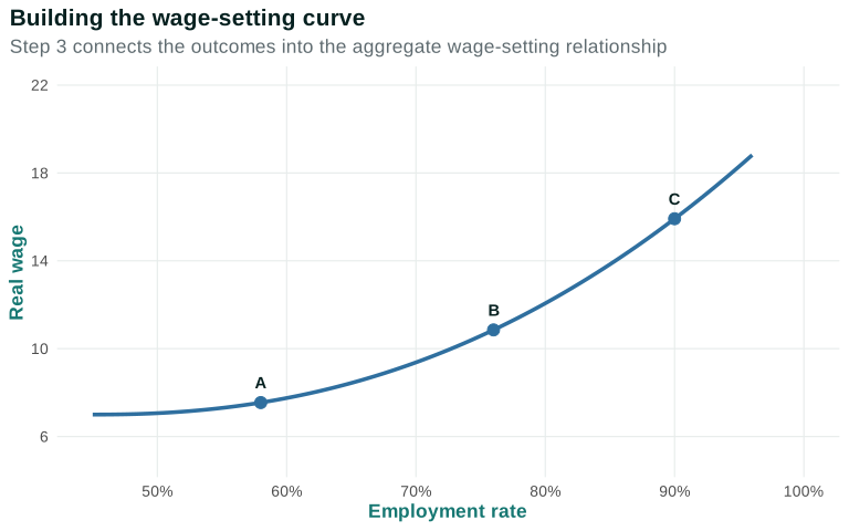
The curve is a relationship among possible outcomes. It is not the economy’s path through time.
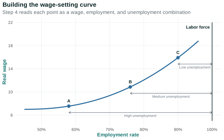
Each point implies both an employment rate and an unemployment gap. Moving from A to C means moving along the same curve: unemployment falls and the real wage firms need to offer rises.
A worker’s next-best alternative
Begin with the whole choice, not the formal label. A person comparing a job offer asks what happens if they decline it or later lose the job. The next-best alternative may include continued search, unemployment insurance, temporary work, study, unpaid care, help from family, or another offer. Economists call the value of that alternative the outside option.
The lowest overall offer a worker would accept depends on that outside option and on the job’s nonwage conditions. This threshold is sometimes called a reservation wage. The term can be useful, but the dollar wage alone is not enough when hours, risk, benefits, treatment, and scheduling differ.
Keeping a job can provide an employment rent
Suppose the value of having the job over a period is 110 and the value of the next-best alternative is 95. The difference—15—is the employment rent. It is the benefit of keeping this job relative to losing it and taking the next-best available course. “Rent” here does not mean a payment to a landlord. It means a benefit above what is required to make the next-best option equally attractive.
Employment rent is not the same for every worker. If finding another acceptable job is quick, the outside option is strong and the rent from keeping the current job may be smaller. If unemployment is likely to last, benefits are limited, savings are low, or another employer is inaccessible, job loss is more costly and the rent may be larger. An employer may therefore possess more authority over a worker whose alternatives are weak, even when both formally agreed to the contract.
Why a firm may not choose the lowest wage
An employment contract is incomplete: it cannot specify and enforce every action, judgment, quality decision, cooperative task, or future contingency. A restaurant manager cannot write a clause for every interaction with a customer. A nurse continually exercises judgment that cannot be reduced to a checklist. A warehouse contract cannot anticipate every safety decision or equipment failure.
The firm therefore cares not only about bringing someone through the door. It cares about recruiting suitable workers, retaining experience, avoiding disruption, and supporting reliable effort and cooperation. Higher pay can sometimes reduce quits, widen the applicant pool, make job loss more costly, or improve the conditions under which people work. These effects are not automatic and need evidence in any particular setting. They explain why the cheapest hourly wage need not minimize labor cost per effective unit of work.
A stylized feasible-offer comparison
| Offer | Real wage | Next-best alternative | Employment rent | Expected effective work units | Wage cost per effective unit |
|---|---|---|---|---|---|
| A | 100 | 95 | 5 | 0.80 | 125.0 |
| B | 110 | 95 | 15 | 1.00 | 110.0 |
| C | 120 | 95 | 25 | 1.03 | 116.5 |
These numbers are illustrative, not estimates. Offer A has the lowest wage but the highest cost per effective unit because recruitment, turnover, or unreliable work is costly in the example. Offer B costs more per hour but less for each expected effective unit. Offer C adds little effective work relative to its higher wage, so its cost per effective unit rises again. In this example, B is the lowest-cost feasible offer.
Now change one condition. Suppose the worker’s next-best alternative rises from 95 to 103 while the three wage offers remain fixed. Employment rent becomes negative at A, 7 at B, and 17 at C. A may no longer recruit or retain the worker. B may remain acceptable but create a smaller advantage to keeping the job. The firm must reconsider the offer if it wants the same recruitment, retention, or effort outcome. CORE mechanism translated through a numerical table
From one firm to the wage-setting relationship
At a low economy-wide employment rate, job finding is generally harder and unemployment risk is greater. At a higher employment rate, more vacancies and alternative offers can strengthen workers’ outside options. Holding the other conditions of the problem fixed, firms generally need to offer a higher real wage to obtain the same recruitment, retention, or motivation advantage. Connecting the feasible offers associated with different employment rates gives the wage-setting relationship.
This relationship summarizes many choices; it is not a contract signed by “the economy.” Firms differ in technology, turnover cost, market power, and management. Workers differ in skills, wealth, care obligations, legal protections, discrimination, and access to collective organization. The curve is a disciplined simplification used to study one common feedback: economy-wide employment affects outside options, which affect feasible wage offers.
In more advanced economics, a wage chosen partly because pay affects retention, effort, or effective labor input is often called an efficiency wage. The label is optional here. The important preparation is the sequence: pay can affect the employment rent; the rent can affect behavior that is not fully contractible; and the firm compares labor cost with effective work. A formal model can write these relationships as functions and find a best response, but the analytical logic is already present in the table.
Application question. What mechanism must be present before the efficiency-wage label adds anything to the analysis?
- The wage is higher than last year
- Pay changes the effective work or continuity the firm expects
- Every action is perfectly enforceable in the contract
Comparing named points on the same relationship
Return to points A, B, and C in the analytical figure. At A, employment is lower and unemployment is higher. Job finding is harder, so the next-best alternative is weaker for many workers. A lower real wage can still create an employment rent large enough for the firm’s recruitment-and-retention problem.
At B, employment is higher. More workers encounter vacancies or credible alternatives, so losing the current job is generally less costly. If the firm offered the same real wage as at A, the employment rent would be smaller. The feasible offer therefore rises. At C, employment is higher again and unemployment lower, so the same reasoning leads to a still higher feasible real wage.
The comparison changes one economy-wide condition—the employment rate—while holding the institutions and the firm’s underlying recruitment-and-retention problem fixed. That is why A, B, and C lie on the same relationship. The points are possible combinations, not dates and not a forecast that the economy automatically travels from A to C.
Now compare a different case. Keep the employment rate at B but strengthen workers’ outside options through a specified institutional change. The feasible real wage rises at the same horizontal position. This is a change in the wage-setting relationship, not a movement from B toward C. Naming the initial and comparison points makes the distinction visible without adding an expert label.
The analytical curve also does not rank the points by social welfare. Higher employment and higher real wages may sound preferable, but the diagram omits hours, job quality, unpaid work, prices, profits, environmental costs, and the distribution of risk. It also does not show whether firms find each combination compatible with their pricing and production choices. Those missing choices are why Chapter 3 needs a separate relationship.
Questions
Review the live step-by-step figure
Question 2.5. Why might a firm offer more than a worker’s reservation wage?
- To make job loss costly enough to support effort and retention
- Because all workers have the same outside option
- Because effort is completely enforceable in court
- To guarantee that unemployment is zero
Exercise
Three feasible offers
Use Figure 2.3 to compare points A, B, and C. For each point, state the relative employment, unemployment, and real wage. Explain why a tighter labor market can require a higher feasible wage.
The model solution is available in the restricted instructor materials.
2.6 Points on the curve and an empirical wage-setting relationship
The most common reading mistake is to call every change a shift. If unemployment falls because economy-wide demand for labor rises while institutions and the recruitment-and-motivation problem are unchanged, the outcome moves along the wage-setting curve. The lower unemployment rate makes workers’ outside options better, and the feasible wage rises.
The model’s claim can be compared with evidence. Figure 2.5 follows the empirical curve reported in TE 2.0 and attributed to Stephen Machin using US Current Population Survey Outgoing Rotation Group microdata for 1979–2019. CORE describes a sample of men aged 26–64 with controls for age, education, race, state, and year, using variation across local labor markets. The current chapter asset is a digitized design placeholder, not yet a reproducible empirical result. TE 2.0 Figure 1.21
Reading the empirical wage-setting figure one step at a time
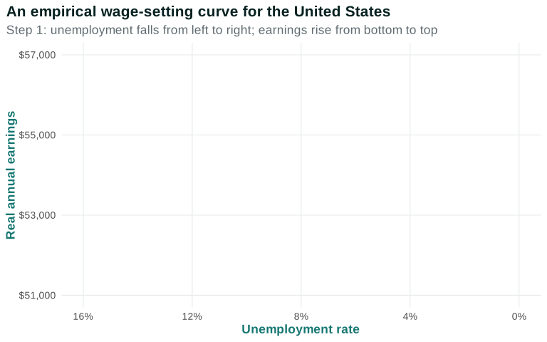
The horizontal axis runs from high unemployment on the left to low unemployment on the right. That makes moving right correspond to higher employment, as in Figure 2.4.
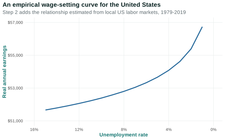
Estimated earnings rise as unemployment falls. The curve becomes steeper at very low unemployment in the published estimate.
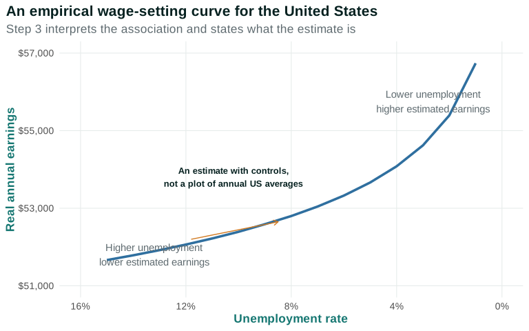
The evidence is consistent with wage-setting logic, but it is not the analytical curve observed directly. The controls and research design matter; other samples, periods, wage measures, and local-area definitions may produce different estimates.
Data-review flag: The plotted line was digitized from the published CORE SVG and remains a design placeholder. Before publication or canonical transfer, obtain and verify the underlying CORE/Machin values, code, or complete specification; otherwise use an independently reviewed CPS re-estimation or a published replacement. Record uncertainty, methods, source, rights, and population limits.
machin_data.csv
Simon Halliday’s earlier BFH textbook repository contains an exact machin_data.csv source file. We have pinned that file in this project for reproducibility and provenance review. Archived BFH source
It appears to be an earlier presentation of the Machin wage-setting estimate, but it is not identical to the current TE 2.0 figure. The archived file has 17 observations spanning unemployment rates from 2% to 18% and reports annual earnings in 2013 dollars. The current TE 2.0 graph has 15 plotted values spanning 1% to 15% and reports earnings in 2019 dollars. The earlier BFH script converts unemployment into an employment rate, which mirrors the horizontal axis without changing the relationship.
For that reason, the live graph above continues to match the current TE 2.0 presentation while the archived file serves as a valuable cross-check. We will not treat the two datasets as interchangeable until the price-base conversion, sample, period, and regression specification are verified.
Data question. Why can the archived values not simply replace the current plotted values?
- Because an employment-rate axis must slope in the opposite economic direction
- Because the files differ in coverage and units and may represent different versions of the estimate
- Because the archived file cannot be reproduced
Analytical and empirical relationships answer different questions
The analytical wage-setting curve summarizes a proposed mechanism: when employment is higher, outside options generally strengthen and the real wage required for recruitment, retention, or effort rises, holding other conditions fixed. The empirical relationship asks whether earnings tend to be higher in tighter US local labor markets after making specified comparisons. Evidence consistent with the mechanism is useful, but it does not turn the analytical curve into something directly observed.
The current plotted asset is provisional. It digitizes points from CORE’s published figure, which attributes the estimate to Stephen Machin and CPS Outgoing Rotation Group data. The chapter can use the figure as a design placeholder while requesting the underlying values, code, or complete regression specification. Publication requires one of three routes: obtain and verify those materials; reproduce a clearly documented estimate from CPS microdata with independent methods review; or substitute a published US wage-curve estimate whose population, outcome, geography, controls, uncertainty, and rights can be taught accurately.
Until that gate is passed, students should not be asked to read precise dollar values from the digitized line. They can still learn the evidence questions: Who is included? Is the comparison across years, places, or people? What has been adjusted for? How is unemployment measured? Does the graph display uncertainty? What alternative mechanisms could produce the pattern?
The current sample description also marks a limitation rather than a universal result. An estimate for men aged 26–64 does not automatically describe women, younger entrants, older workers, people outside the labor force, or groups facing different discrimination and care constraints. A later version should either justify this population for the teaching question or pair it with evidence that broadens the comparison.
Questions
Review the live step-by-step figure
Question 2.6. In Figure 2.4, why does unemployment fall from left to right?
- To make the empirical figure comparable with the employment-rate direction in Figure 2.3
- Because unemployment can never rise
- Because the figure is a national time series
- Because earnings are measured in nominal dollars
Exercise
Analytical curve and empirical estimate
Compare Figures 2.3 and 2.4. Identify one shared prediction, two differences in construction, and one reason the empirical estimate does not by itself prove the entire wage-setting mechanism.
The model solution is available in the restricted instructor materials.
2.7 When the wage-setting curve shifts
A shift occurs when the feasible wage changes at the same employment rate. Consider an improvement in workers’ fallback position. More adequate unemployment insurance, faster job search, a more attractive set of alternative jobs, or stronger collective bargaining may reduce the cost of losing the current job. To recruit, retain, or motivate workers at the original employment rate, firms must offer more.
Reading the wage-setting shift one step at a time
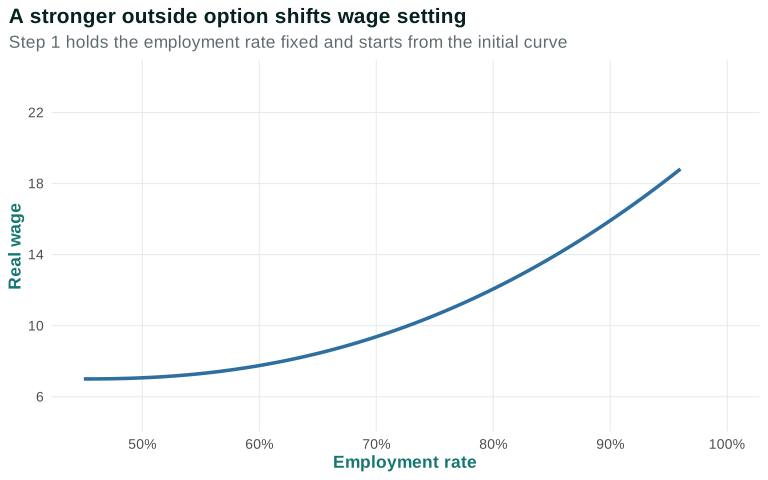
Choose an employment rate and ask which real wage is feasible on the initial curve.
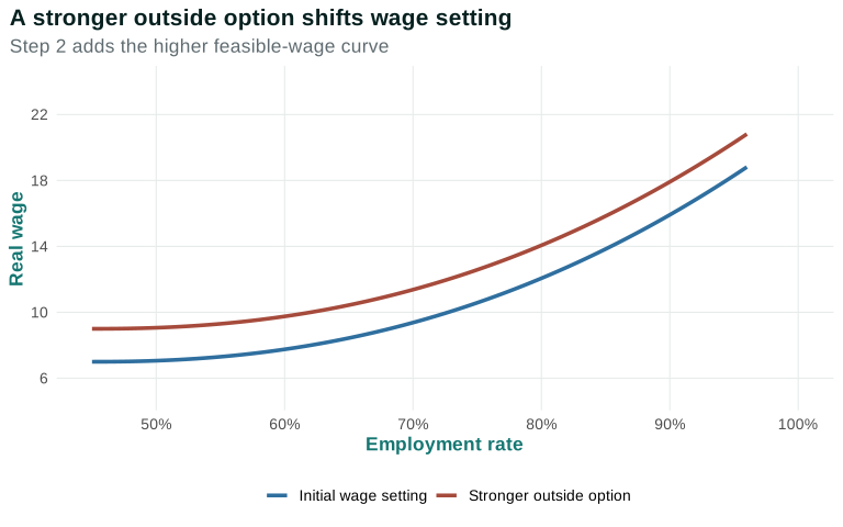
At every employment rate, the second curve associates wage setting with a higher real wage.
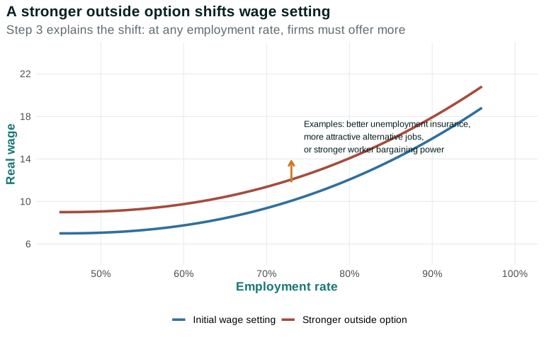
The figure does not say that every stronger outside option has the same effect, or that employment is unchanged after the economy adjusts. It isolates the first step: which condition changes, whose choices change, and why the feasible wage differs at the same employment rate.
Monitoring, workplace norms, turnover costs, discrimination, and bargaining institutions can also change wage setting. Some changes may affect productivity or the composition of jobs at the same time. Chapter 4 will treat institutions as more than one-dimensional curve shifters.
Change one condition, then trace the choices
The upward shift in the figure is a first comparison, not a complete prediction of the economy’s final employment and wage. Begin at a named employment rate. Change one institution or condition. Ask how the worker’s next-best alternative or the firm’s recruitment-and-retention problem changes. Compare the feasible real wage at the same employment rate. Only after that comparison should we ask about wider adjustments, many of which require the price-setting relationship introduced in Chapter 3. CORE mechanism translation
Case 1: unemployment insurance
More adequate unemployment insurance can raise the material value of the outside option during an eligible unemployment spell. A worker may be able to search longer for a suitable match instead of accepting the first available job. At the original employment rate, a firm seeking the same retention or motivation advantage may need to offer a higher real wage or improve other job conditions.
This is not a claim that every recipient searches less or that employment must fall. Eligibility, benefit duration, household needs, local vacancies, and search requirements differ. Insurance can also improve matching and stabilize spending. Chapter 2 isolates the outside-option channel; later chapters add other channels and economy-wide feedback.
Case 2: bargaining rights and collective organization
When workers can bargain collectively, they may obtain information, representation, grievance procedures, and bargaining power that an individual worker lacks. Those institutions can raise the wage or improve conditions feasible at a given employment rate. They can also change worker voice, retention, training, and productivity. A bargaining-only change and a productivity change are distinct mechanisms. Chapter 4 will keep them separate when combining wage setting with the rest of the model.
Collective organization also changes whose preferences enter the decision. A firm has legal and organizational authority to direct work within the employment relationship. A union or worker organization can constrain that authority and give workers a collective exit or voice option. Treating this merely as a number added to a curve would hide the institution that changes the choices.
Case 3: monitoring and worker voice
More intensive monitoring can make some actions easier for an employer to observe. In a narrow model, this can reduce how much the firm needs to rely on the cost of job loss to support a required action. But monitoring itself uses resources and can affect privacy, trust, stress, safety reporting, and turnover. It may raise measured compliance while reducing cooperation that cannot be easily measured.
Worker voice is different. Employees often possess information about workflow, customers, hazards, and equipment. Institutions that make it safer to speak can improve decisions and reduce costly turnover. If voice raises productivity, that is not simply an outside-option shift. The chapter records the distinction now so that Chapter 4 does not reverse or conflate the channels.
Case 4: unequal buffers and constrained mobility
A stronger outside option is not only a policy parameter. Wealth, family support, housing, transportation, health coverage, disability accommodations, credentials, citizenship, and discrimination can determine whether a person can wait, move, search, or risk conflict with an employer. Two workers paid the same wage can therefore have different employment rents and different exposure to unemployment risk.
These dimensions intersect. Education can open some jobs, but a degree does not erase racial discrimination, care responsibilities, disability barriers, citizenship constraints, or unequal wealth. Class position includes wage dependence, ownership, authority, collective organization, credentials, and intergenerational resources. The wage-setting model is useful precisely because it directs attention to alternatives and power, but a single curve cannot display all of them.
Reading the shifted curve responsibly
At point D on the original curve, record the employment rate and feasible real wage. Keep that employment rate fixed. Introduce one stronger outside-option condition and locate point E vertically above D on the new curve. Explain which actor’s constraint changed and why the firm’s feasible offer is higher. Do not claim that the economy remains at E. We do not yet know how firms’ prices, profits, hiring, or output respond.
Questions
Review the live step-by-step figure
Question 2.7. Which change is a shift rather than movement along the wage-setting curve?
- Employment rises while the recruitment-and-motivation relationship is unchanged
- A stronger outside option raises the feasible wage at the same employment rate
- Unemployment falls as employment rises
- A point is relabeled from A to B
Exercise
Move or shift
Classify each as movement along WS or a possible shift: lower unemployment with unchanged institutions; more generous unemployment insurance; easier monitoring; better alternative jobs. For each shift, explain the first-step mechanism.
The model solution is available in the restricted instructor materials.
2.8 What Chapter 2 has built—and what comes next
We began with measured labor-market states and flows, then connected employment, hours, and productivity to output and nominal pay to purchasing power. Those measures established what must be explained. The wage-setting relationship supplied the first behavioral building block: firms’ feasible wage offers depend on workers’ outside options, and those outside options depend partly on employment across the economy.
The wage-setting curve alone does not determine employment or the real wage. It tells us what wage is consistent with recruitment and motivation at each employment level. Chapter 3 adds firms’ price-setting choices and the division of output per worker between wages and profits. Only then can we ask where both sets of choices are mutually consistent.
National averages also conceal unequal access to jobs, outside options, bargaining power, and income. UOE Micro’s matching-market analysis supplies one bridge from classification to unequal opportunity. UOE Micro Ch. 10 Chapter 4 will ask how institutions and power change both the size and distribution of the gains from employment.
The chapter has also established a method for reading macroeconomic models. Start with people and institutions, not a curve. Identify goals and constraints. Use accounting to organize the quantities. Build the behavioral choice numerically or verbally. Aggregate only after the individual mechanism is clear. When one condition changes, compare named points and say what is being held fixed. End by stating what the model leaves out and who bears the risk.
Seeing the principles in action
| Principle | Example | Everyday Economics |
|---|---|---|
| Interdependence principle — focal | A graduate’s opportunities and a firm’s feasible wage both depend on the hiring and search choices made throughout the labor market. | The same résumé or wage offer can receive different responses in a booming labor market and a recession. |
| Doing the best you can principle | Workers decide whether to search, accept a job, study, or provide care given income needs, time, transport, information, and available jobs. | Someone may stop searching because another month of search is costly even when paid work remains their preferred outcome. |
| Rules of the game principle | BLS definitions determine recorded labor-market states, while unemployment insurance and bargaining rules change workers’ outside options and can shift wage setting. | A more adequate fallback may change which job offers workers can reject and which wages firms can feasibly offer. |
| Trade-offs and opportunity costs principle — focal | Accepting a job now provides earnings but may end a search for a better match; studying or caregiving uses time that could have been paid work. | The opportunity cost of one more week of job search depends on savings, benefits, and the offers currently available. |
| Principle of gains from cooperation and conflict of interest | A productive job match can benefit worker and employer, while they may conflict over wages, hours, security, and working conditions. | A job offer can create gains for both sides even when neither side receives everything it wants. |
| Principle of individual and societal interests | A firm’s decision to cut hours can protect its finances while reducing household income and aggregate output. | What is sensible for one employer during a downturn may deepen the downturn when many employers act similarly. |
| Principle of aggregation and feedback — focal | Individual transitions determine aggregate employment, while aggregate unemployment feeds back into workers’ outside options and firms’ feasible wage offers. | One firm’s vacancy is local; widespread hiring changes unemployment and can alter the wage every firm must consider. |
Skills and learning objectives
- Interpreting labor market statistics
- Reading a flow chart
- Reading an analytical graph
- Reading and interpreting an empirical graph (and its terms)
- Adjusting a model in response to economic or institutional changes
- Understanding the difference between causality and correlation
- Defining important economic terms
- Applying the interdependence and opportunity cost and trade-offs principles
Concepts to learn
- Employment, unemployment, the labor force, stocks, and flows
- Employment, hours, labor productivity, and aggregate output
- Nominal wages, price indexes, real wages, and purchasing power
- Reservation wage, no-shirking wage, and employment rent
- Feasible wage offers and the wage-setting curve
- Employment and unemployment as points on wage setting
- Empirical wage-setting estimates
- Movement along a curve and shifts in a curve
Glossary
Chapter 2 terms
employed
Classified as having done paid work during the survey reference period, or as having a job from which one was temporarily absent.
See also: unemployed; outside the labor force.
unemployed
Without a job, available for work, and actively seeking work under the statistical definition, or on qualifying temporary layoff.
See also: employed; outside the labor force; labor force.
outside the labor force
Neither employed nor classified as unemployed; this group includes many students, retirees, caregivers, and people not actively searching.
See also: employed; unemployed; labor force.
labor force
The number of people classified as employed plus the number classified as unemployed.
See also: employed; unemployed.
stock
A quantity measured at a point in time, such as the number of people employed in a given month.
See also: flow.
flow
A quantity measured over an interval, such as hires, quits, or transitions from unemployment to employment during a month.
See also: stock.
labor productivity
Output per unit of labor input, measured here as output per hour or output per worker.
nominal wage
A wage measured in current dollars, without adjusting for the prices of goods and services.
See also: real wage; price index.
real wage
A wage adjusted by a price index so that changes reflect purchasing power rather than dollars alone.
See also: nominal wage; price index.
price index
A statistical measure that summarizes the prices of a specified basket relative to a base period.
See also: nominal wage; real wage.
reservation wage
The reservation wage summarizes the value of not accepting the current job, including income while unemployed, expected time to another offer, and the expected quality of alternative work. Workers can therefore have different reservation wages even when they have similar skills.
See also: outside option; employment rent; wage-setting curve.
outside option
The next-best alternative available if a current interaction or agreement ends.
See also: reservation wage; employment rent.
employment rent
The net benefit a worker receives from keeping a job compared with the worker’s next-best alternative.
See also: outside option; incomplete contract.
incomplete contract
A contract that cannot specify or enforce every action each party will take in every possible circumstance.
See also: employment rent; outside option.
wage-setting curve
The wage-setting curve slopes upward because higher employment means lower unemployment and generally better outside options for workers. A point on the curve combines a feasible real wage with an employment and unemployment level; a shift changes the feasible wage at the same employment rate.
See also: outside option; employment rent; reservation wage.
Flashcards
What is the difference between a labor-market stock and a flow?
A stock is measured at a point in time; a flow records movement over an interval.
How do employment, hours, and productivity combine to produce output?
Output equals workers times average hours per worker times output per hour.
Why can the feasible wage rise when unemployment falls?
Workers can find alternatives more easily, so firms may need a higher wage to recruit, retain, and motivate them.
Movement along WS or a shift?
A change in employment with the relationship unchanged is movement along WS; a change in the feasible wage at the same employment rate is a shift.
Questions
Question 2.8. Why does Chapter 2 not yet determine equilibrium employment?
- The wage-setting curve contains no real wage
- A second relationship is needed to identify which wage and employment combination is mutually consistent
- Employment cannot be measured
- Firms never set prices
Exercise
Build the next question
State what the wage-setting curve determines and what it does not. Then explain why a price-setting relationship is needed before the model can identify an equilibrium real wage and employment rate.
The model solution is available in the restricted instructor materials.