Inflation, Cost of Living, and Distribution
Public working draft: This AI-assisted chapter draft is open for coauthor revision. Household examples are teaching cases, not estimates. Figures, quantitative claims, source rights, and distributional conclusions still require human review.
Central question: Why can the same inflation rate feel so different across households?
By the end of this chapter, you should be able to: distinguish a price level from its rate of change; construct and interpret a simple fixed-basket price index; explain why CPI, PCE, core inflation, and the GDP deflator answer different questions; calculate an inflation rate and a real-wage change; compare household-specific spending baskets; trace expected and unexpected inflation through nominal contracts; and identify who bears inflation risk when prices, wages, benefits, debts, and rents adjust at different times.
7.1 Prices rose; inflation fell
In 2023, a student working at a grocery store could hear that inflation was falling and still find groceries, rent, and transit more expensive than before the pandemic. The student’s hourly wage might also have risen, but not at the same date or by the same percentage as every price. A retired neighbor could face a different combination: a fixed mortgage or no mortgage, a Social Security adjustment each January, and a larger share of spending on health care. “Inflation is down” did not answer either person’s budget question.
Both the news report and the household experience can be accurate. The apparent contradiction comes from confusing a level with its rate of change. The level tells us how high an index is. The rate tells us how quickly that index is rising or falling. A car can still be moving forward after it slows down; similarly, a price index can keep rising after inflation falls.
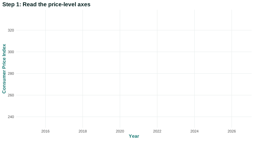
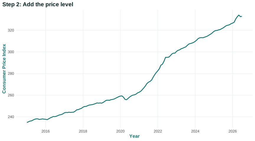
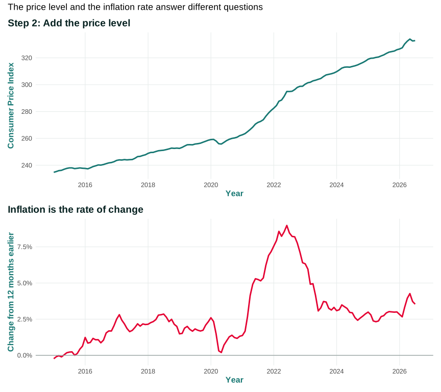
Figure 7.1 begins with the US Consumer Price Index for All Urban Consumers. The horizontal axis records months since 2015. In the upper panel, the vertical axis is the CPI price level, an index summarizing prices at a point in time, with the benchmark set by BLS to an average of 100 in 1982–84. The benchmark does not mean that a particular basket cost exactly $100 in those years. It provides a common scale for comparing the price level across dates. In the lower panel, the vertical axis is the percentage change in that index from twelve months earlier.
Open the live step-by-step figure
First compare the two panels during 2021 and 2022. The price level rises steeply, so the twelve-month inflation rate also rises. Next compare the inflation peak with later months. The lower-panel rate falls, but it remains positive for much of the period. The upper-panel index therefore keeps rising, only less rapidly. Disinflation is a fall in the inflation rate while it may remain positive. Deflation is a fall in the overall price level.
The figure is descriptive. It records average price change for a defined population and basket. It does not show which households bought which goods, whether wages kept pace, why prices rose, or who had the power and resources to adjust. It also cannot establish whether demand, supply, expectations, margins, or policy caused the change. Chapter 8 will investigate those mechanisms. This chapter first asks what the headline itself measures and how a national average connects to unequal household positions. TE 2.0 inflation measurement sequence
The central question follows: Why can the same inflation rate feel so different across households? To answer it, we must construct an index from prices and expenditure weights, then examine the contracts and institutions that connect the index to purchasing power.
Questions
Review the live step-by-step figure
Question 7.1. If inflation falls from 8% to 3%, then…
- the price level must fall
- prices rise more slowly
- all prices fall 5%
- purchasing power always rises
Exercise
Level and rate
Use Figure 7.1 to explain how inflation can fall while the cost of a fixed basket continues to rise.
The model solution is available in the restricted instructor materials.
7.2 Constructing a price index
A price statistic begins with people purchasing particular goods and services, not with one object called “the price level.” A household sees rent, bread, electricity, bus fare, tuition, medication, and thousands of other prices. A statistical agency needs a procedure for selecting products and outlets, comparing like with like, and combining price movements into one measure.
The Consumer Price Index is produced by the US Bureau of Labor Statistics. The CPI-U is designed to represent price change for purchases by urban consumers. BLS uses household expenditure information to construct weights, samples prices across locations and outlets, replaces items when necessary, and adjusts for some quality changes. These are technical operations, but they are also institutional choices that determine what the index means. BLS CPI methods
The population comes first. CPI-U covers urban consumers, representing most of the US population, while CPI-W uses expenditure patterns for households meeting wage-earner and clerical-worker criteria. Neither index begins by following one permanent set of families. The goal is to estimate price change for a statistical population. A student comparing the headline with a personal budget should therefore ask two separate questions: Is the index well designed for its population? How closely does this student’s basket resemble the population weights?
Price collection also requires a sampling frame. Consumers purchase at supermarkets, online retailers, hospitals, landlords, gas stations, and many other outlets. BLS cannot record every transaction. It samples geographic areas, outlets, items, and services, then uses statistical procedures to combine the resulting price observations. A sampled price is supposed to refer to a comparable product and transaction. Discounts, package sizes, taxes, insurance arrangements, and outlet changes can complicate that comparison.
Quality change is especially difficult. Suppose a laptop costs 10 percent more but has a faster processor, longer battery life, and better screen. Treating the full dollar increase as pure inflation would ignore improved characteristics. Treating it as entirely improved quality would ignore any price increase for comparable computing services. Statistical agencies use several methods, including direct comparisons and models of product characteristics, to separate quality from price where possible. The adjustment is an estimate, not an assertion that consumers value every feature equally.
Housing illustrates another conceptual decision. Renters purchase housing services through rent. Owner-occupiers consume housing services from an asset they own, but a house purchase is also an asset transaction. The CPI represents owner-occupied housing primarily through an estimate of the rent the home would command, not the current sale price of houses. This distinction is sensible for a consumption price index, yet it can surprise a first-time buyer watching home prices and mortgage rates.
The phrase “cost of living” can also exceed what a price index measures. Maintaining the same standard of living may require changing quantities when prices change, finding new suppliers, accepting different quality, or spending more time. A fixed-basket index asks how much the old quantities would cost. A cost-of-living index asks how much expenditure is needed to reach a comparable level of well-being under new prices. The second question depends on available substitution and on what counts as equivalent well-being.
Substitution is not costless. If beef becomes expensive, a household may buy chicken; if a preferred brand rises, it may switch brands. But a wheelchair-accessible apartment, prescribed medication, nearby childcare, or reliable car for a night shift may have no close substitute. Statistical substitution can describe average behavior without implying that every household can avoid the increase. A lower measured cost after substitution may include a real loss of convenience, quality, identity, time, or access.
New goods create the opposite problem. A product that did not exist in the base period has no base quantity. Smartphones combined services once purchased separately, while streaming replaced some physical media. The welfare gain from a new product can be larger than its observed price decline, yet estimating that gain requires assumptions about demand and quality. The index is not defective because it cannot directly observe well-being; it is limited to a defined measurement task.
Measurement error has distributional consequences when contracts and public programs use an index. If an index overstates the relevant price change, indexed payments can rise faster than the intended purchasing-power target. If it understates the change for a vulnerable population, real benefits can erode. That is why index selection, methods, and governance are part of public policy rather than a neutral afterthought.
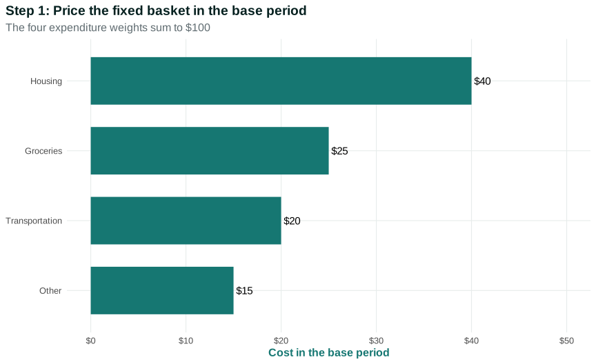
Begin with a transparent fixed basket. Imagine that its base-period cost is $100:
| Category | Base-period expenditure | Later price change | Cost of the same quantities later |
|---|---|---|---|
| Housing | $40.00 | 12% | $44.80 |
| Groceries | $25.00 | 8% | $27.00 |
| Transportation | $20.00 | 20% | $24.00 |
| Other goods and services | $15.00 | 4% | $15.60 |
| Total | $100.00 | — | $111.40 |
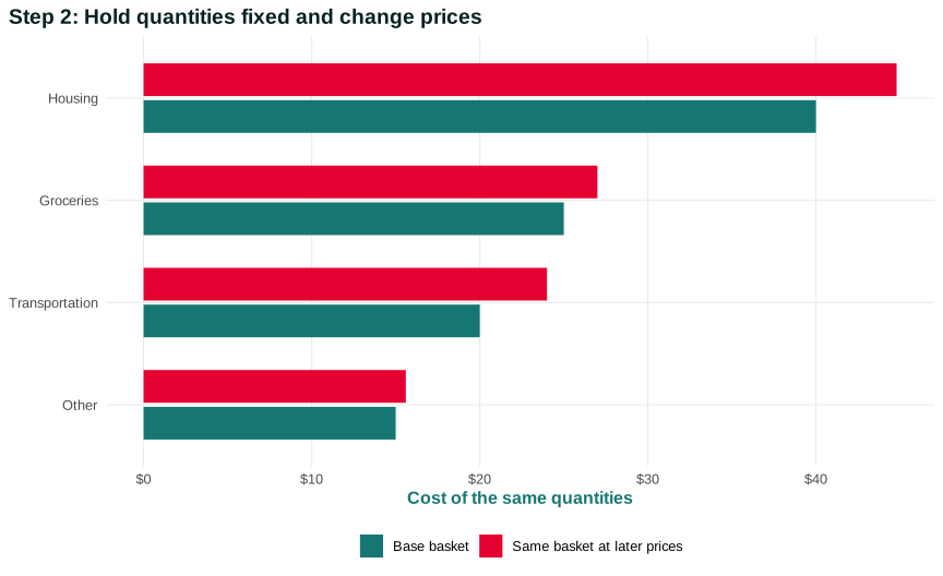
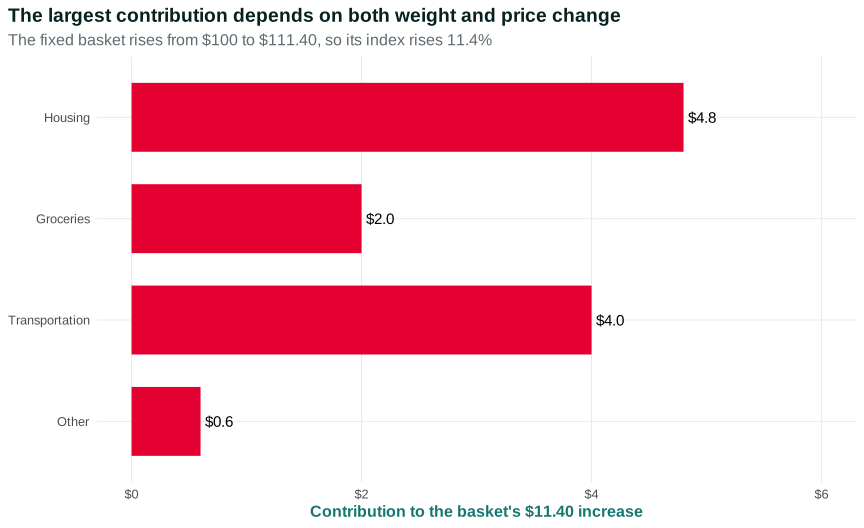
The quantities are held fixed in this exercise. Housing has a weight of 40 percent because it accounts for $40 of the $100 base basket. A 12 percent housing-price increase adds $4.80. Transportation has a smaller weight but a larger price increase, so it adds $4.00. The total later cost is $111.40.
Figure 7.2 teaches the calculation in three stages. First read the base-period weights. Then compare the cost of the same quantities at later prices. Finally compare each category’s contribution to the total increase. A category affects the index through both its weight and its price movement.
Open the live step-by-step figure
If the index equals 100 in the base period, it equals 111.4 later. That does not mean every listed price rose 11.4 percent. It means the cost of this fixed combination rose 11.4 percent. Nor does the example claim that an actual household spends these amounts. Its purpose is to make the aggregation visible.
Real indexes confront harder questions. Households substitute when relative prices change. A product can improve or deteriorate in quality. New products appear and old ones disappear. Rent is directly observed for renters, but owner-occupied housing provides a service without a monthly rent payment to a landlord. Prices can differ across cities, stores, contract types, and purchase dates. No single method makes those problems vanish.
The Rules of the game principle applies because a trustworthy index depends on transparent statistical authority, methods, funding, professional independence, and opportunities for scrutiny. Method changes do not automatically make an index political manipulation. They can correct a problem or adapt to new markets. But users must know what changed before comparing values across time.
Math Extension 7.2.1: A fixed-basket formula
Let \(q_{i0}\) be the base-period quantity of item \(i\), \(p_{i0}\) its base-period price, and \(p_{it}\) its price in period \(t\). A simple fixed-basket index is
\[ P_t = 100 \times \frac{\sum_i p_{it}q_{i0}}{\sum_i p_{i0}q_{i0}}. \]
The numerator is the cost of buying the base quantities at period-\(t\) prices. The denominator is their base-period cost. In the table, the ratio is \(111.40/100\), so \(P_t=111.4\). Official indexes use more sophisticated sampling, aggregation, linking, and quality-adjustment procedures. The formula prepares you to read those methods; it is not a reproduction of the full CPI system.
Questions: Which part of the formula holds quantities fixed? What would change if households substituted toward categories whose relative prices rose less?The basket calculation establishes how a weighted average is constructed. It still does not tell us how fast the index changed over a specified interval. That is the next step.
Questions
Question 7.2. Why are price-index weights important?
- They determine how individual price changes affect the aggregate
- They make all household baskets identical
- They eliminate quality change
- They measure unemployment
Exercise
Build two baskets
Construct renter and homeowner baskets with different weights and calculate how the same price changes produce different experienced inflation.
The model solution is available in the restricted instructor materials.
7.3 From an index to an inflation rate
The inflation rate is the percentage change in a specified price index over a stated interval. If an index rises from 120 to 126, the change is six index points. The inflation rate is
\[ \frac{126-120}{120}\times 100 = 5\%. \]
Six index points and 5 percent are different statements. A percentage change divides by the starting level. This matters when comparing periods whose index levels differ.
The interval also matters. Suppose a price index moves as follows:
| Date | Index | Change from prior month | Change from twelve months earlier |
|---|---|---|---|
| January last year | 120.0 | — | — |
| December last year | 125.5 | 0.4% | 4.6% |
| January this year | 126.0 | 0.4% | 5.0% |
| February this year | 125.7 | −0.2% | 4.4% |
The index can fall in February even though it remains far above January of the prior year. Monthly inflation is negative in February, while twelve-month inflation remains positive. Neither statement is false. They compare different dates.
Base effects can make a twelve-month rate move even when the latest monthly change is ordinary. The twelve-month calculation compares today’s index with the index exactly one year earlier. When an unusually large increase drops out of that comparison window, twelve-month inflation can fall sharply even if the current month is not especially low. Conversely, an unusually low starting value can raise the twelve-month rate. Reading the underlying index levels prevents the denominator from disappearing from the story.
Compounding matters across months. If a price index rises 1 percent in one month and another 1 percent in the next, the two-month increase is \(1.01\times1.01-1=2.01\) percent. Adding monthly rates gives a close approximation for small changes, but not an exact result. An annualized monthly rate raises the monthly growth factor to the twelfth power. A 1 percent monthly increase annualizes to about 12.7 percent—not because analysts predict twelve identical months, but because they express the pace on a common annual scale.
Percentage points are used to compare rates, not levels. If inflation falls from 8 percent to 3 percent, it declines by 5 percentage points, or 62.5 percent relative to its initial rate. The first description is usually clearer. If a category’s weight rises from 10 to 12 percent of the basket, its share rises by 2 percentage points and by 20 percent relative to the initial share. Careful language prevents a large-sounding relative change from being confused with its contribution to the overall index.
News reports may quote monthly changes, twelve-month changes, quarterly annualized rates, or averages. Seasonal adjustment may remove recurring patterns such as holiday purchases or regular fare changes. Annualizing asks what a short-period rate would imply if repeated for a year; it does not assert that it will repeat. Always identify the interval, transformation, and adjustment before comparing two rates.
Inflation can slow because some prices rise less rapidly, because prices in a few categories fall, or because the composition and weights of the index change. A lower rate does not reverse all prior increases. If the price level rises 8 percent and then 2 percent, the two-year increase is approximately 10.2 percent, not zero and not exactly 10 percent, because the second change applies to the higher level.
Students and policymakers often care about a cumulative question: how much did the cost of a defined basket change over several years? A twelve-month inflation rate is not enough. The correct comparison uses the price-index levels at the start and end of the full interval. This is why Figure 7.1 shows both level and rate.
The arithmetic distinguishes descriptions. It does not explain why the numerator changed. A higher index could reflect demand pressure, energy costs, rents, supply constraints, margins, wages, taxes, or many combined mechanisms. Before explaining causes, we must also decide which index matches the question.
Questions
Question 7.3. An index rising from 120 to 126 implies inflation of…
- 5%
- 6%
- 6 percentage points
- 126%
Exercise
Calculate inflation
Calculate inflation when an index rises from 120 to 126; distinguish percent from percentage-point change.
The model solution is available in the restricted instructor materials.
7.4 Different measures answer different questions
There is no one inflation measure that answers every question. Measures differ because their populations, scopes, formulas, and institutions differ. Choosing among them should follow the question, not the desired headline.
| Measure | Main population or scope | Weight/formula idea | Useful question | Important limitation |
|---|---|---|---|---|
| CPI-U | Out-of-pocket purchases by urban consumers | BLS consumer expenditure weights; modified fixed-basket approach | How are prices paid by urban consumers changing? | Not a personal index; excludes some spending made on households’ behalf |
| CPI-W | Urban wage earners and clerical workers | A different population’s expenditure weights | What statutory index is used for Social Security COLAs? | Population does not match all beneficiaries |
| PCE price index | Consumption spending by and on behalf of households and nonprofit institutions serving households | BEA chain-type Fisher approach | How are prices across personal consumption expenditures changing? | Broader scope and revisions can make it less intuitive for a household receipt |
| GDP deflator | Prices of domestically produced final output | Current production composition | How have prices of domestic final production changed? | Not a consumer cost-of-living measure; includes investment and government output, excludes imports |
| Core CPI or core PCE | Corresponding index excluding food and energy | Same institutional base with selected categories removed | Is broader inflation moving apart from volatile food and energy components? | Households still buy food and energy; “core” is an analytical filter, not their budget |
BEA explains the CPI–PCE difference through formula, weights, scope, and other measurement effects. PCE includes some spending made on behalf of households, including parts of health care that may be paid by employers or government. CPI focuses more directly on household out-of-pocket purchases. PCE weights also respond differently when consumers substitute across categories. BEA CPI–PCE comparison
The GDP deflator answers a production question. An imported phone enters consumer spending but is not domestic production, so the import price affects a consumer index differently from the GDP deflator. Conversely, a price increase for domestically produced machinery can affect the GDP deflator without being part of a household consumption basket.
“Core” inflation is commonly used to look through food and energy volatility. It does not mean those prices are unimportant or unreal. A large food or gasoline increase can dominate a household budget and alter wage demands, expectations, and spending. The exclusion is a diagnostic choice: analysts ask whether price changes are broadening or likely to persist beyond volatile categories.
Consider four users. A union preparing wage negotiations may begin with CPI because members care about consumer purchasing power, then examine member-specific housing, health, and transportation costs. A central bank studying persistent consumption inflation may emphasize PCE and core PCE because of their scope, formula, and place in its stated goal. A business revising a long-term contract may choose a narrow input-price index rather than a broad consumer measure. A researcher comparing nominal GDP with real GDP uses the GDP deflator because the relevant basket is domestic final production. The appropriate index follows the economic object being deflated.
Revision practices also differ. The non-seasonally-adjusted CPI is generally not revised after publication except for correction, while seasonal factors can be updated. PCE estimates draw on national-account data that are revised as more complete information arrives. Revisions can improve the historical estimate while complicating real-time policy evaluation. An analyst asking what policymakers knew in a particular month should preserve the vintage available then; an analyst reconstructing the best current history may prefer revised data.
Geographic comparisons require additional care. A higher CPI level for one city does not necessarily mean that city is more expensive than another because most CPI series are designed to compare price change over time within an area, not absolute cost levels across places. Regional price parities and carefully matched price-level data answer cross-place questions. The index number printed beside two cities can share a base without creating a valid cost-of-living ranking.
Measures can also diverge because weights change. If consumers substitute away from a category whose relative price rises, a chain-weighted measure can place less weight on that category sooner than a fixed-basket calculation. That may better represent changing consumption, but it can answer a different question from “How much more would the old basket cost?” Neither question is illegitimate. The key is to state which one the measure answers.
Statistical independence is a public institution. Price measures influence contracts, tax brackets, benefit payments, central-bank decisions, and political arguments. Producers must publish methods, document revisions, protect respondent confidentiality, and withstand pressure from actors who gain or lose when the measured rate changes. Users also have responsibilities: cite the series, preserve vintages where relevant, distinguish seasonal from nonseasonal values, and avoid choosing a measure after seeing which one supports a desired conclusion.
No agency can eliminate judgment. Classifying a new product, estimating owner-equivalent rent, handling a temporary missing price, or adjusting quality requires rules and evidence. The appropriate accountability is not to demand a judgment-free index. It is to make judgments professional, reproducible, reviewable, and aligned with the published concept.
Institutions attach consequences to particular indexes. Tax parameters, private escalation clauses, wages, rents, and benefits may use different rules. Social Security’s automatic cost-of-living adjustment is tied by law to the CPI-W and compares third-quarter averages. The adjustment protects benefits with a lag and cannot make every beneficiary’s personal basket identical to the statutory population. Social Security COLA rules
Data Extension 7.4.1: CPI, PCE, and a statutory COLA
Use the BLS CPI methods overview, the BEA CPI–PCE comparison, and the Social Security COLA description to complete a three-row source table. For each source, record the institution, population or scope, weight/formula description, update or revision practice, and one policy use.
Then answer two questions. First, which measure would you choose to deflate an urban worker’s out-of-pocket consumption budget, and what would it omit? Second, which measure would you choose to evaluate the prices of all domestically produced final output, and why would it treat imports differently?
Questions: Why is disagreement between CPI and PCE not automatically evidence that one agency made an error? Why might a retiree’s experienced price change differ from the CPI-W-based COLA even when the statutory calculation is correct?A measure is defensible when its construction matches the claim. Switching between CPI, PCE, and the GDP deflator without stating the question produces apparent precision without conceptual clarity. The next section asks what happens when we use one of these measures to evaluate wages and household purchasing power.
Questions
Question 7.4. Which index is designed around consumer expenditures?
- Consumer Price Index
- Unemployment rate
- Nominal GDP
- Union membership rate
Exercise
Choose an index
Choose between CPI, PCE, and GDP deflator for three questions and justify the population and scope.
The model solution is available in the restricted instructor materials.
7.5 Real wages and household purchasing power
A worker is paid in dollars but consumes goods, services, housing, time, and public provision. A real wage adjusts a money wage by a price index to measure purchasing power. If an hourly wage rises 4 percent while a relevant price index rises 6 percent, the worker’s purchasing power falls by roughly 2 percent. The exact calculation compares ratios:
\[ \text{real-wage change}=\frac{1.04}{1.06}-1\approx -1.9\%. \]
The approximation subtracts inflation from nominal wage growth. It is useful for small changes, but the ratio is more accurate. The conclusion also depends on the chosen deflator. A consumer price index answers a purchasing-power question. An output price or GDP deflator answers a different question.
Average real-wage growth does not establish that every worker gained. Workers enter and leave employment, change hours, and work in industries with different wage paths. Benefits, tips, bonuses, taxes, commuting costs, scheduling, and job risk matter. If low-wage workers disproportionately lose jobs, the average wage among those still employed can rise even when many workers are worse off. The numerator, denominator, and population all require attention.
There are several defensible real-pay questions. One compares average hourly earnings with a consumer price index. Another follows the same workers over time. A third asks whether total weekly earnings kept pace after hours changed. A fourth includes employer health insurance or retirement contributions. A fifth adjusts disposable income after taxes and transfers. These measures can move differently because they describe different resources and populations.
Suppose a worker’s hourly wage rises from $20 to $21, a 5 percent increase. If the relevant index rises from 125 to 131.25, also 5 percent, hourly purchasing power is unchanged by that calculation. But if weekly hours fall from 35 to 30, real weekly earnings fall substantially. If the worker begins paying more for employer health coverage or commuting, disposable purchasing power can fall further. “Real wages were flat” is not a complete description of living standards.
Public services complicate the household budget in the other direction. A free school meal, subsidized transit pass, public college grant, or expanded health benefit can increase capabilities without appearing as a lower market price in the household’s basket. A cut in public provision can force a household to purchase a market substitute. Chapter 1’s living-standards framework therefore remains relevant: resources, distribution, capabilities, and institutional access cannot be compressed into one consumer price index.
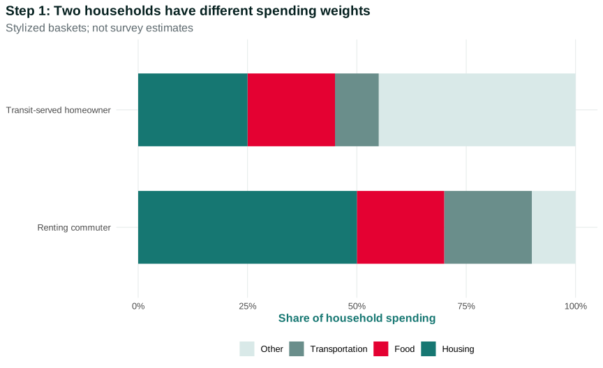
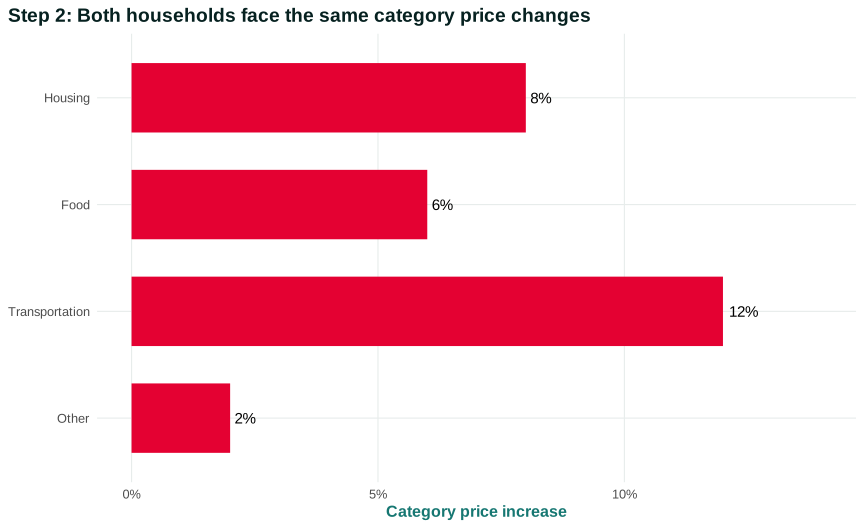
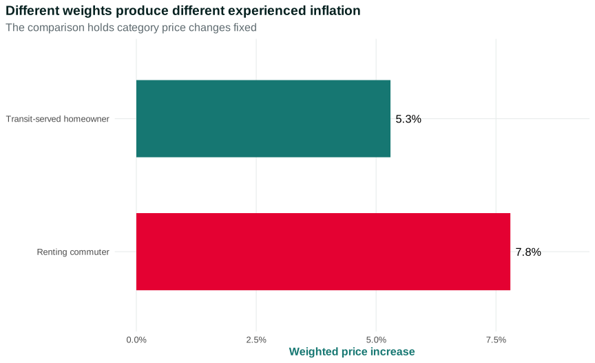
Households also buy different baskets. Figure 7.3 holds four category price changes fixed and compares two stylized households. The “renting commuter” devotes a larger share to housing and transportation. The “transit-served homeowner” devotes less to those categories and more to other goods and services. These labels describe the example only; they are not estimates for all renters or owners.
Open the live step-by-step figure
The renting commuter’s weighted increase is 7.8 percent; the other household’s is 5.3 percent. The only changed condition is the basket. We have not changed the category price movements. That discipline tells us what the comparison establishes: expenditure weights can create different experienced inflation. It does not establish the size of actual renter–owner differences.
BLS Consumer Expenditure Surveys document how expenditure patterns vary with income, household composition, housing tenure, race, age, place, and other characteristics. Those patterns reflect both preferences and constraints. A low-income household may devote a high share to necessities because little income remains after housing, food, utilities, and transportation. A person with a disability may face unavoidable medical or transportation expenses. Rural households may have fewer substitution options than households near public transit. Citizenship and access to programs can affect public and private prices. BLS Consumer Expenditure Surveys
Class is not just an income quintile. Ownership affects whether a housing payment is fixed, variable, or implicit; wealth affects the capacity to draw on assets; authority affects wage and price setting; wage dependence affects exposure to job loss; and collective organization affects bargaining over nominal pay. These positions intersect with race, gender, disability, place, and citizenship because past and current institutions shape homeownership, wealth, occupations, care responsibilities, credit access, and public services.
The Trade-offs and opportunity costs principle appears in household responses. A family can switch brands, postpone care, move, commute farther, work more, draw down savings, or borrow—but each option has a cost and some are infeasible. Saying “households substitute” without naming the available alternatives can hide hardship.
Different baskets explain part of unequal experience. Timing adds another layer. Wages, benefits, rents, and loan payments are governed by contracts that may adjust before, after, or not at all when prices change.
Questions
Question 7.5. Wages rise 4% and relevant prices rise 6%. The approximate real-wage change is…
- +10%
- +2%
- -2%
- 0%
Exercise
Real wage
Calculate the approximate real-wage change for 4% nominal wage growth and 6% inflation, then explain why a household-specific result may differ.
The model solution is available in the restricted instructor materials.
7.6 Expected and unexpected inflation
Inflation changes real outcomes most directly when nominal promises were set earlier. A nominal contract specifies dollar payments: a wage, rent, pension, loan repayment, or supply price. The contract also assigns timing and authority. Who can reopen it? When? Under what formula? What happens if one party cannot pay?
Expected inflation is the price increase people anticipate when making a decision. If workers, firms, borrowers, and lenders all expect 2 percent inflation, they may incorporate it into nominal wages, prices, interest rates, and budgets. Expectations are uncertain and heterogeneous; they are not facts about the future.
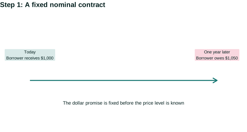
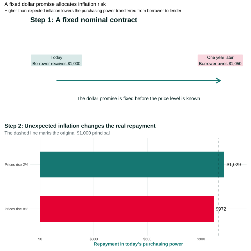
Unexpected inflation is the difference between the price change built into a decision and what occurs. Suppose a borrower receives $1,000 and promises $1,050 one year later. The dollar repayment does not change when the price level changes. Its purchasing power does.
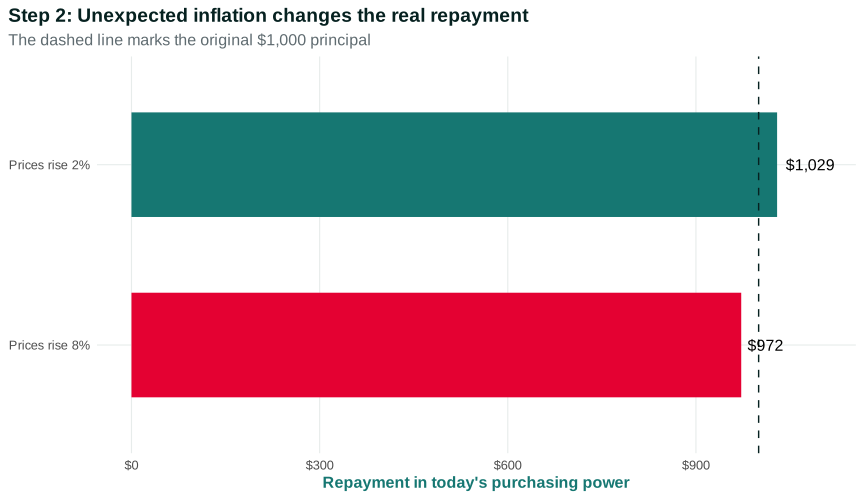
Figure 7.4 compares price-level increases of 2 and 8 percent. At 2 percent inflation, the $1,050 repayment is worth about $1,029 in today’s purchasing power. At 8 percent, it is worth about $972. Higher-than-expected inflation transfers less purchasing power to the lender and leaves the borrower repaying with dollars that buy less.
Open the live step-by-step figure
The model isolates inflation risk. It holds the nominal repayment fixed and changes the price level. It omits default, taxes, fees, variable interest rates, changes in borrower income, and the fact that lenders may themselves owe fixed nominal debts. An actual distributional conclusion requires balance sheets, contract terms, and income adjustments.
Now change one condition at a time. If the loan carries an adjustable rate, policy tightening can raise the nominal payment, offsetting some of the debtor’s gain from past inflation. If the borrower’s income does not rise with prices, even a lower real debt burden may coexist with cash-flow distress. If the lender is a pension fund owing partly indexed benefits, lower real repayment can affect beneficiaries rather than a single wealthy creditor. Balance-sheet chains turn a two-person example into an institutional network.
Expectations affect the nominal term when the contract begins. If both parties expect higher inflation, the lender may require a higher nominal interest rate. The borrower then does not receive an automatic windfall from inflation that was already priced into the agreement. The redistribution arises from the difference between actual and expected inflation, along with taxes, default risk, and other contract features.
Wage contracts allocate risk differently. An employer may promise a fixed nominal raise, a cost-of-living adjustment, or a reopen clause if inflation crosses a threshold. Full backward-looking indexation protects purchasing power after measured inflation but can transmit an earlier shock into later wages. A forward-looking agreement depends on forecasts and bargaining power. A worker without a formal contract may receive quicker discretionary changes—or no protection at all.
Rent contracts combine price protection with renewal risk. A one-year lease fixes nominal rent during the term, helping the tenant when market rents rise unexpectedly. At renewal, the landlord may attempt a large catch-up increase, subject to law, vacancy conditions, and the tenant’s moving costs. A rent regulation can limit adjustment, but maintenance, housing supply, property values, and access rules affect who ultimately bears costs. The phrase “renters lose from inflation” is too simple without this timing.
The same logic applies unevenly elsewhere. A worker with a one-year wage agreement loses purchasing power when prices unexpectedly rise before renegotiation. A firm may gain if it can raise output prices before wages or input contracts adjust. A renter with a fixed lease is temporarily protected from a market-rent increase; a landlord faces rising costs until renewal. A benefit indexed annually adjusts with a lag. An adjustable-rate borrower can face rising nominal payments when monetary policy responds.
Indexation changes the timing and allocation of risk. A contract can automatically link payments to a price index, but the index choice and adjustment frequency matter. Full and immediate indexation may protect one party while transmitting inflation quickly to another. Partial or delayed indexation allows purchasing power to change between revisions. Institutions never remove the real question of who absorbs a loss when the economy has fewer resources.
Math Extension 7.6.1: Nominal interest, expected inflation, and expected real return
For small rates, the expected real interest rate is approximately the nominal interest rate minus expected inflation. A more exact one-period relation is
\[ 1+r = \frac{1+i}{1+\pi^e}, \]
where \(i\) is the nominal interest rate and \(\pi^e\) expected inflation. The formula describes the expected purchasing-power return when the contract is set. The realized real return uses actual inflation and can differ. Chapter 11 will return to interest, saving, and borrowing with balance sheets and default risk.
Questions: Why does the expected real return differ from the realized return? Which party bears the surprise under a fixed-rate loan?Expected inflation can be built into contracts; surprises redistribute; and adjustment timing varies. We can now combine baskets, contracts, and economic positions to understand why inflation is not a uniform tax.
Questions
Question 7.6. Unexpected inflation tends to benefit which party in a fixed nominal debt?
- The borrower, if nominal income rises
- The lender automatically
- Neither party ever
- Only government
Exercise
Nominal contract
Analyze an unexpected inflation increase for a fixed-rate borrower, lender, worker, and benefit recipient.
The model solution is available in the restricted instructor materials.
7.7 Inflation redistributes
Inflation changes an average price level, but it also occurs through changing relative prices. Food, energy, rent, used cars, wages, profits, benefits, taxes, and interest payments do not move at the same time or by the same percentage. Distribution depends on what a person owns, owes, sells, buys, and has authority to renegotiate.
| Economic position | Nominal term or price exposure | Potential protection | Important risk |
|---|---|---|---|
| Wage-dependent worker | Wage schedule and hours | Frequent bargaining, indexation, tight labor market, union organization | Prices rise before pay; job loss during anti-inflation adjustment |
| Firm owner | Output prices, wages, input costs, debt | Price-setting power, diversified assets, fixed-rate debt | Input and wage costs rise faster than output price; demand falls |
| Renter | Lease, utilities, moving costs | Fixed lease during term, rent regulation, housing assistance | Renewal shock, eviction risk, few substitutes |
| Homeowner borrower | Fixed or adjustable mortgage, maintenance, taxes | Fixed-rate nominal debt can lose real value | Adjustable payment, insurance/tax increase, income loss |
| Lender or bondholder | Fixed nominal repayment | Inflation premium, short maturity, indexed asset | Unexpected inflation reduces real repayment |
| Benefit recipient | Statutory or program adjustment formula | Automatic indexation | Lag, mismatched index, eligibility or administrative barriers |
The table does not label groups as permanent winners and losers. Many people occupy several positions. A worker can own a retirement account and a home, owe a mortgage, and receive a public benefit. A small business owner can be a debtor with little price-setting power. The net effect depends on the full balance sheet, budget, contract calendar, and employment response.
Consider a household with two wage earners, a fixed-rate mortgage, childcare costs, a car loan, and retirement savings. Unexpected inflation reduces the real burden of fixed nominal debts, which helps. But childcare, food, insurance, and repair prices may rise before wages. If monetary tightening reduces one worker’s hours, the household can lose income even while its mortgage debt becomes smaller in real terms. Retirement assets may rise or fall depending on interest rates and portfolio composition. There is no single sign without tracing each position.
Now compare a renter receiving disability benefits and working part time. Rent may be fixed for several months and then jump at renewal. Benefits may be indexed annually, while work income depends on hours and program rules. Medical and transportation needs may limit substitution. A national inflation average is relevant to benefit policy, but it cannot replace analysis of accessible housing, health coverage, program administration, and the person’s actual budget.
A distribution table should therefore have at least four columns: the resource or obligation, the nominal adjustment rule, the timing of adjustment, and the actor with authority. Adding “likely gain or loss” before those columns encourages stereotypes. The mechanism determines incidence.
Inflation incidence can also change within a category. Two renters may have the same current rent but different renewal dates. Two homeowners may have fixed mortgages originated at different rates, or one may rent out part of the property. Two workers may receive the same nominal raise but face different hours, commuting distances, care obligations, or eligibility for public programs. Economic position is more informative than a broad demographic label by itself.
Race and gender matter through institutions and accumulated positions, not as alternative explanations competing with class. Discrimination in housing and credit, occupational segregation, unequal wealth, care responsibilities, immigration rules, and neighborhood infrastructure shape baskets, contracts, and capacity to adjust. A distributional analysis should identify those channels and evidence rather than merely list group averages.
Inflation uncertainty has a cost separate from a known average rate. Households and firms must spend time comparing prices, renegotiating contracts, forecasting costs, holding liquidity, or postponing commitments. Those costs are unequal. A large firm can employ specialists and diversify suppliers; a small firm or low-income household may have less information, bargaining power, and financial buffer. Predictability can therefore matter even when indexation protects average purchasing power.
Power matters because not everyone can adjust a nominal claim equally. A firm with loyal customers and limited competition may raise prices quickly. A worker bargaining alone may wait a year for a raise. A union can coordinate bargaining but still face strike costs and unemployment risk. A landlord in a tight market may raise rent at renewal; a tenant cannot instantly replace housing. Government chooses indexation rules and eligibility; the central bank influences demand, interest rates, and employment.
The Principle of aggregation and feedback connects these positions. One household’s higher wage is a firm’s cost and the household’s income. One firm’s price is another firm’s input cost and its owner’s revenue. Higher interest payments are a debtor’s cost and a creditor’s income. When many actors try to protect purchasing power, their responses alter demand, costs, expectations, and policy.
This chapter has established four distinctions. A price level is not an inflation rate. A national index is not a personal receipt. Nominal growth is not real purchasing-power growth. Expected inflation written into a contract is not the same as an unexpected change after the contract is set.
These distinctions prevent common mistakes, but they do not yet explain why inflation begins or persists. A price index can show when and where prices changed. It cannot by itself distinguish demand pressure from a supply shock, or determine whether wages, margins, expectations, and policy propagated the change. Chapter 8 builds those mechanisms and asks what evidence could tell them apart.
Before moving on, apply a final measurement checklist. First, name the index and its population or scope. Second, identify the dates and whether the claim concerns a level, monthly change, twelve-month change, or annualized pace. Third, separate nominal from real resources using a defensible deflator. Fourth, identify household weights, contracts, and adjustment timing. Fifth, state what the evidence describes and which causal questions remain open.
Suppose a headline says “Wages beat inflation.” The checklist asks: which workers and wage measure; hourly or weekly earnings; which inflation index; which start and end dates; average or median; continuously employed workers or changing composition; before or after taxes and benefits; and whether subgroup baskets differed? The headline may be correct after those questions, but its meaning becomes narrower and more useful.
Suppose another headline says “Inflation cost the average household $X.” Turning an index change into dollars requires a reference expenditure level and basket. The result can illustrate scale, but it is not a bill sent to every household. Households with different spending, housing tenure, debt, geography, and access to public services face different changes. A careful analysis reports assumptions and a distribution, not only an average.
Finally, measurement itself does not determine whether inflation is acceptable or which policy should respond. That judgment involves employment, output, distribution, predictability, contracts, public goals, and alternative instruments. Reliable indexes make those debates possible; they do not resolve them. Chapter 8 supplies causal mechanisms, and Chapters 9–10 examine policy authority and trade-offs.
Seeing the principles in action
| Principle | Example | Everyday Economics |
|---|---|---|
| Interdependence principle | Prices, wages, benefits, rents, debts, and taxes connect household budgets to firms and government. | A fuel price increase changes commuting costs and delivery costs. |
| Doing the best you can principle | Households substitute, delay, borrow, or work more given income and available alternatives. | A renter cannot substitute away from housing as easily as from a brand of cereal. |
| Rules of the game principle — focal | Statistical rules define the basket, weights, quality adjustments, population, and index formula. | A headline index is not any one household’s receipt. |
| Trade-offs and opportunity costs principle — focal | Responding to higher prices requires giving up consumption, time, savings, or future borrowing capacity. | Driving farther for cheaper groceries uses time and gasoline. |
| Principle of gains from cooperation and conflict of interest | Contracts coordinate exchange while unexpected inflation redistributes between workers, firms, borrowers, and lenders. | A fixed nominal payment becomes easier for a borrower when incomes rise. |
| Principle of individual and societal interests | Protecting one’s own real income can shift costs onto others. | A successful price or wage increase changes another party’s purchasing power. |
| Principle of aggregation and feedback — focal | A price index aggregates unequal baskets, while wage-price-policy responses feed back into inflation. | Your experienced inflation can differ from the national average. |
Skills and learning objectives
- Distinguishing a price level from inflation
- Calculating an inflation rate
- Comparing price indexes
- Calculating a real wage change
- Analyzing inflation’s distributional effects
Concepts to learn
- Price level and price index
- Inflation disinflation and deflation
- CPI and alternative price measures
- Real wages and household baskets
- Expected and unexpected inflation
- Borrowers lenders and nominal contracts
- Distributional effects of inflation
Glossary
Chapter 7 terms
price level
An index summarizing the prices of a representative basket or set of goods and services at a point in time.
See also: inflation rate; price index.
inflation rate
The percentage increase in a price index over a stated period.
See also: price level; disinflation; deflation.
deflation
A fall in the general price level, corresponding to a negative inflation rate.
See also: inflation rate; disinflation.
price index
A weighted measure that combines many prices relative to a benchmark.
See also: price level.
disinflation
A decrease in the inflation rate while it may remain positive and the price level may continue to rise.
See also: inflation rate; deflation.
real wage
A money wage adjusted for a relevant price index to measure purchasing power.
See also: inflation rate.
expected inflation
The rate of price increase that people anticipate and may incorporate into contracts, plans, and interest rates.
nominal contract
An agreement that fixes or schedules payments in dollars rather than directly guaranteeing purchasing power.
See also: expected inflation; inflation rate.
Flashcards
Does falling inflation mean prices are falling?
No. Positive but lower inflation means prices are rising more slowly; deflation means the price level falls.
What is a real wage?
A money wage adjusted by a price index to measure purchasing power.
Why is experienced inflation unequal?
Households buy different baskets, face different contracts, and have unequal ability to substitute, borrow, or protect income.
Questions
Question 7.7. Why can households experience different inflation?
- They buy different baskets and face different adjustment options
- The national index is fabricated
- Only income matters
- Inflation affects only borrowers
Exercise
Inflation distribution map
Choose one price shock and map effects through class, place, contracts, and household baskets without assuming everyone loses equally.
The model solution is available in the restricted instructor materials.