Aggregate Demand and the Multiplier

Public working draft: This AI-assisted chapter draft is open for coauthor revision. Its Google Doc remains canonical. The analytical figures are teaching models rather than empirical multiplier estimates; all empirical claims and policy applications require human review.
Central question: How can one person’s decision to spend less reduce other people’s income?
By the end of this chapter, you should be able to: distinguish the GDP identity from behavioral spending decisions; trace how an initial spending change becomes income and generates later rounds; calculate and interpret a simple multiplier; explain how taxes, imports, transfers, and automatic stabilizers alter feedback; compare households’ capacity to smooth consumption; analyze investment and expectations; and explain why individually prudent saving can reduce aggregate income.
6.1 When spending disappears
During the Great Recession, a construction worker could lose hours because homebuilding collapsed. During the pandemic recession, a restaurant server could lose hours because face-to-face activity stopped abruptly. In both cases, the first income loss did not stay with one person. A worker who postponed a car repair reduced a mechanic’s revenue. The mechanic might delay buying equipment. A supplier then received fewer orders. A local government might collect less tax revenue just as more residents needed help.
These chains are easy to describe after the fact and difficult to measure causally. Output, employment, consumption, and investment move together during recessions. The initiating events differ, and several mechanisms operate at once. We therefore begin with a descriptive comparison and then build a deliberately simple model of one feedback channel.
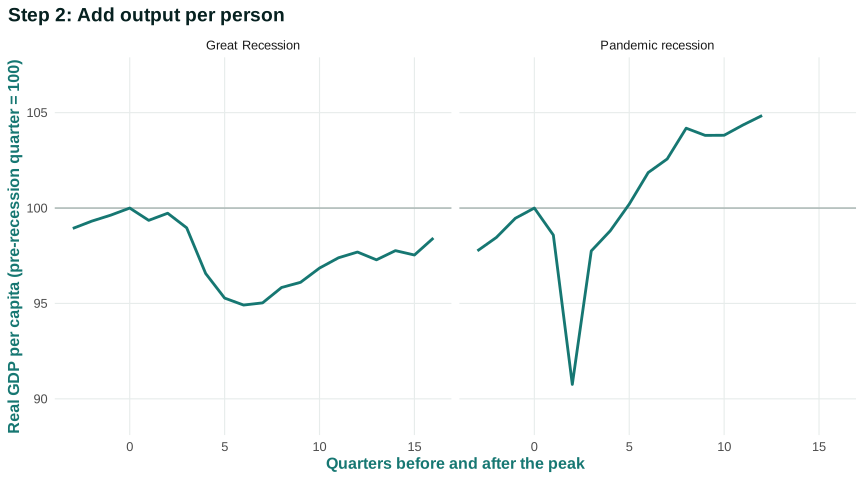
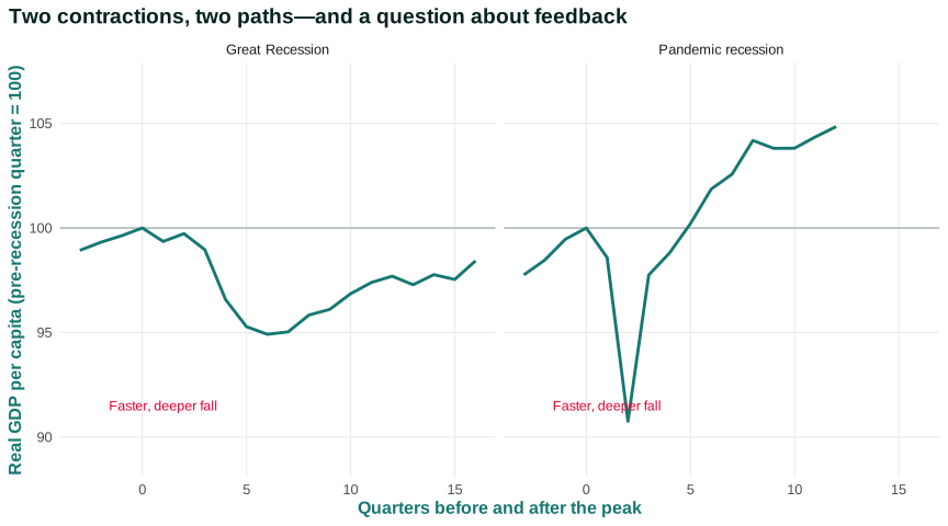
Figure 6.1 places real GDP per person around the Great Recession and pandemic recession on comparable indexes. In each panel, the pre-recession quarter equals 100. The horizontal axis measures quarters before and after that baseline, rather than calendar dates. The common vertical scale lets us compare depth and speed.
Open the live step-by-step figure
The Great Recession path falls more gradually and remains depressed for longer in the displayed window. The pandemic path plunges and rebounds much more sharply. Indexing makes proportional movements comparable, but it discards their different calendar dates, institutional settings, and starting levels. The figure does not show that a single demand shock caused either recession.
Chapter 5 established an accounting fact: realized expenditure, income, and output are equal views of completed activity. That equality remains true in expansion and recession. Yet an identity cannot tell us why activity moved. To explain a contraction, we must introduce plans, constraints, timing, and responses.
Aggregate demand is total planned spending on domestically produced goods and services under stated economic conditions. It includes consumption, investment, government purchases, and exports net of the import content of spending. It is not simply the right side of the GDP identity renamed. Planned spending depends on income, expectations, wealth, credit, taxes, transfers, public decisions, foreign demand, and prices. Realized expenditure equals output after firms and households have adjusted; planned expenditure can initially differ from what firms expected to sell.
Our central question is therefore about a sequence: How can one person’s decision to spend less reduce other people’s income? We begin with one transaction, then let recipients respond, then ask how institutions and unequal resources change the chain. TE 2.0 multiplier sequence
Questions
Review the live step-by-step figure
Question 6.1. What does Figure 6.1 show?
- Two contractions with different depth and speed
- Both recessions had the same cause
- Demand never matters
- Output is nominal
Exercise
Compare contractions
Use Figure 6.1 to compare depth and speed, then explain why the comparison does not identify a demand shock by itself.
The model solution is available in the restricted instructor materials.
6.2 Spending becomes income
Follow one payment
Suppose Maya receives a temporary $500 payment and spends $300 at a locally owned appliance store. Her expenditure is the store’s revenue. The store uses some revenue to pay workers, suppliers, rent, taxes, and interest; the remainder may become profit. Each recipient then makes a new decision about spending.
The accounting statement is immediate: Maya’s realized $300 purchase is revenue elsewhere. The behavioral statement is not. We cannot infer how much the store’s workers, owners, or suppliers will spend next. Their choices depend on whether the income increase is expected to persist, whether bills are due, how much liquid wealth they have, what credit is available, and how uncertain they feel.
| Stage | Actor | Added receipts | Immediate decision | Amount spent domestically next |
|---|---|---|---|---|
| Initial | Maya | $500 transfer | Spend, save, or repay debt | $300 |
| Revenue | Appliance store | $300 sale | Pay workers/suppliers, retain cash | not fixed by accounting |
| Income | Workers, owners, suppliers | claims on $300 revenue | Spend, save, pay tax, import, or repay debt | behavioral outcome |
The marginal propensity to consume is the fraction of an additional dollar of disposable income that a household spends on consumption in the model. “Marginal” means additional. It is not the share of total income spent, the share of wealth spent, or a moral characteristic of a household.
Suppose a household’s disposable income rises from $2,000 to $2,100 per month and consumption rises from $1,900 to $1,975. The additional income is $100 and the additional consumption is $75, so the household’s MPC over this change is 0.75. The remaining $25 increases saving or reduces debt. The average propensity to consume would compare total consumption with total income; that is a different calculation.
Why households respond differently
A student with $50 in a checking account and a rent payment due may spend a large share of an added dollar. A high-wealth household may save much of it. But wealth alone does not determine response. A household may have a house and retirement account but little cash. Credit limits, debt payments, family obligations, medical needs, immigration status, benefit eligibility, and expectations about future income all affect feasible choices.
Empirical research uses tax rebates, stimulus payments, benefit changes, and other income changes to estimate spending responses. Results vary with the size and timing of the payment, the spending category, household liquidity, expectations, and research design. The model’s single MPC is therefore a teaching simplification. It represents a response under stated conditions, not a permanent biological constant.
The timing matters too. A recipient can spend immediately, several months later, or use the payment to repay debt and increase spending only when borrowing capacity improves. A retailer can add inventory before placing new orders. A producer can meet higher demand from existing inventories before raising output. The equality of realized spending and income does not force every response into the same week.
Planned and realized spending
Suppose firms produced goods expecting sales of $10 million, but households planned only $9 million of purchases. The unsold $1 million is recorded as unintended inventory investment. The accounts still balance: realized investment is higher than firms planned. But the inventory surprise gives firms a reason to reduce future orders and production.
This distinction explains why the identity cannot be the causal theory. Plans can be inconsistent. Inventories, production, employment, prices, and future plans adjust until realized outcomes are mutually compatible. In the simple model below, we focus on quantity adjustment: firms meet demand at given prices when capacity is available, then revise production when spending changes.
From household behavior to an aggregate consumption relationship
To build the model, imagine adding the consumption plans of many households at each possible level of aggregate disposable income. Some consumption does not depend closely on current income: people must eat, maintain housing, and meet contractual payments, and they may finance those purchases from savings or borrowing. Other consumption rises as current disposable income rises. Economists often summarize the relationship as a baseline amount plus an induced amount that depends on income.
| Aggregate disposable income | Baseline consumption | Added consumption at MPC 0.75 | Total planned consumption |
|---|---|---|---|
| $0 | $200 | $0 | $200 |
| $400 | $200 | $300 | $500 |
| $800 | $200 | $600 | $800 |
| $1,200 | $200 | $900 | $1,100 |
The $200 baseline is an assumption for the table, not a claim that a zero-income society can consume indefinitely. It could represent spending financed from earlier saving, credit, transfers, or wealth over a limited period. The slope—$75 of additional consumption for each $100 of additional income—is the MPC. Separating the baseline from the response helps students see which part changes when confidence, wealth, credit, or public benefits change.
Aggregating does not remove heterogeneity. The same aggregate relationship can result from different distributions of income and different household MPCs. If income shifts toward households likely to spend more of an added dollar, planned consumption can rise without a change in total income. Conversely, debt repayment or increased precautionary saving can reduce current consumption even when income is unchanged. The aggregate relationship is behavioral and conditional, not a definition.
We now have the behavioral link needed for feedback: recipients spend a fraction of added income. The next section follows repeated rounds and asks where the process ends.
Questions
Question 6.2. The marginal propensity to consume is…
- the share of total wealth spent
- the share of an added dollar of disposable income spent
- an accounting identity
- equal for every household
Exercise
Unequal MPCs
Explain why a liquidity-constrained renter and a wealthy household may spend different shares of an added $500.
The model solution is available in the restricted instructor materials.
6.3 The multiplier process
From an initial order to repeated rounds
Suppose a business receives a new $100 order for domestically produced equipment. Assume, for now, that prices are fixed, firms have spare capacity, every additional dollar of production becomes domestic income, and recipients spend 75 percent of each added dollar on domestic output. These assumptions isolate the feedback mechanism.
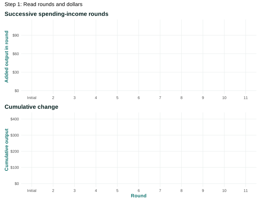
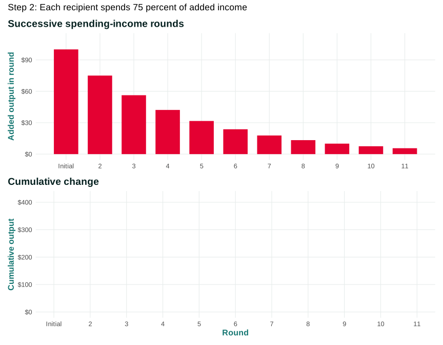
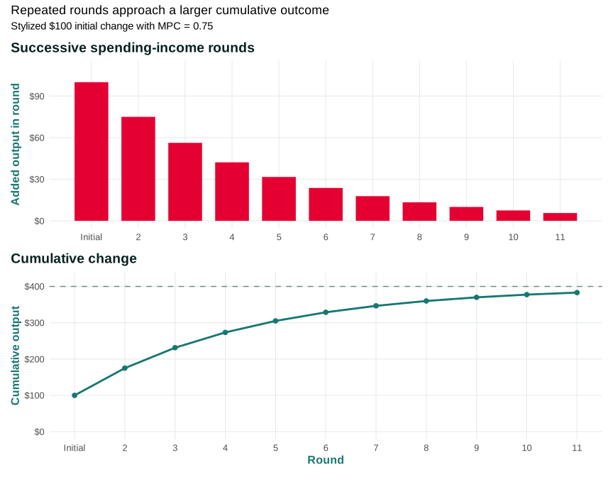
The first $100 is the initial spending change. It raises the equipment producer’s revenue and income generated by $100. Recipients then spend $75. That $75 becomes income to a second group, who spend $56.25. The process continues with smaller rounds.
| Round | Added income in the round | Induced consumption, MPC = 0.75 | Leakage from the next round | Cumulative output change |
|---|---|---|---|---|
| Initial | $100.00 | $75.00 | $25.00 | $100.00 |
| 2 | $75.00 | $56.25 | $18.75 | $175.00 |
| 3 | $56.25 | $42.19 | $14.06 | $231.25 |
| 4 | $42.19 | $31.64 | $10.55 | $273.44 |
| 5 | $31.64 | $23.73 | $7.91 | $305.08 |
A leakage is income not passed into the next round of domestic consumption in the simplified chain. Saving is one leakage from current consumption. Taxes and imports add others when we extend the model. “Leakage” is a role in this mechanism, not a judgment that saving, taxes, or imports are bad.
Figure 6.2 turns the table into a stepped figure. The coral bars show each round, which becomes smaller because only 75 percent is respent. The teal line shows the cumulative change, which approaches a limit.
Open the live step-by-step figure
The multiplier is the total change in equilibrium output divided by the initial spending change. In this stripped-down example, the successive rounds sum toward $400, so the multiplier is 4. The $400 is not created in one transaction. It is the sum of the initial $100 plus later rounds generated as recipients respond.
Math Extension 6.3: The geometric-series multiplier
With an MPC of \(c\), the rounds are \(\Delta A\), \(c\Delta A\), \(c^2\Delta A\), and so on. If \(0<c<1\), their limiting sum is
\[\Delta Y = \Delta A(1+c+c^2+\cdots)=\frac{1}{1-c}\Delta A.\]
The simple multiplier is therefore \(1/(1-c)\). This result follows from the model’s assumptions; it is not an accounting identity and is not an estimate of a particular policy’s effect.
Questions: What happens to the limiting multiplier when \(c\) rises from 0.75 to 0.80? Which real-world leakages make the one-parameter formula incomplete?Adjustment toward a compatible outcome
Another way to understand the endpoint is to compare planned spending with current production. If planned spending exceeds current output and inventories fall unexpectedly, firms have a reason to increase production. Higher production generates income; higher income induces consumption; the gap narrows. If planned spending is below production, inventories accumulate unexpectedly and firms cut production.
The endpoint is an equilibrium in planned expenditure and output under the model’s conditions. It does not mean every household or firm is satisfied, that unemployment is absent, or that the economy is at full capacity. It means firms no longer experience the particular inventory surprise that would lead them to change production.
Why the adjustment takes time
The rounds in the table are logical stages, not necessarily equal calendar periods. A restaurant can respond to a lost reservation within hours. A manufacturer may notice inventories only after a monthly report. A construction firm may already be committed by contract. Workers who lose hours can reduce some purchases immediately but cannot instantly leave a lease or sell a car. Timing depends on contracts, information, and adjustment costs.
Authority also shapes the path. Managers decide production and staffing; lenders can refuse working capital; landlords and utilities can enforce payment; governments determine benefit eligibility and procurement. The multiplier is often drawn as a mechanical series of arrows, but each arrow summarizes someone’s decision under an institution. If a firm keeps workers despite a short sales decline, income feedback is delayed or reduced. If it dismisses workers immediately, the feedback is faster and risk shifts to households and public insurance.
Inventories provide a temporary buffer. A retailer can meet a demand increase from existing stock without immediately raising production. The inventory decline then signals suppliers to increase later orders. During a demand fall, unintended inventory accumulation may precede layoffs. Data recorded in one quarter can therefore combine current spending with production decisions initiated earlier.
The logic also works in reverse. A $100 fall in investment can produce a larger fall in output if lost income leads to further consumption cuts. The model is symmetric only because its assumptions are symmetric. In a real crisis, borrowing constraints, bankruptcy, price cuts, supply disruption, and policy responses can make contractions and expansions different.
Add taxes and imports one leakage at a time
The simple multiplier of 4 assumes that the only amount leaving each next round is household saving. Suppose instead that recipients pay 20 percent of added income in net taxes, spend 10 percent of consumption on imports, and consume 75 percent of added disposable income. We should calculate the sequence rather than attach every leakage to the identity mechanically.
Starting from $100 of added domestic income, a 20 percent tax response leaves $80 of added disposable income. Consuming 75 percent produces $60 of added consumption. If 10 percent of that purchase is imported, $54 becomes the next round of domestic income. The feedback fraction for this example is 0.54, and the next round is much smaller than the $75 in the one-leakage example.
This arithmetic clarifies why open economies, tax systems, and household saving behavior affect the multiplier. It does not imply that taxes or imports reduce well-being. Taxes finance institutions and insurance; imports provide goods, competition, and inputs; saving can support resilience and investment. A leakage is simply a dollar that does not become the next round of the particular domestic-consumption chain being modeled.
We have so far treated the fraction not consumed as one generic leakage. Government, trade, and fiscal rules give those flows distinct actors and consequences.
Questions
Question 6.3. With MPC 0.75, the simple multiplier is…
- 0.75
- 1.33
- 4
- 7.5
Exercise
Multiplier rounds
With an MPC of 0.75 and a $100 initial spending increase, calculate the first four rounds and the simple limiting multiplier.
The model solution is available in the restricted instructor materials.
6.4 Government, trade, and automatic responses
Purchases, taxes, transfers, and imports enter differently
Government purchases create direct demand for currently produced goods and services. Taxes reduce disposable income relative to pre-tax income. Transfers increase recipients’ disposable income but are not themselves purchases of current output. Imports satisfy domestic spending with foreign production, so they do not create the same next round of domestic income.
These distinctions come from Chapter 5’s accounting, but their effects here are behavioral. A $100 government purchase is an initial demand for output. A $100 transfer affects demand only as recipients spend it. A $100 tax change affects demand according to how households and firms respond. A $100 increase in imports can reflect strong domestic spending rather than economic weakness.
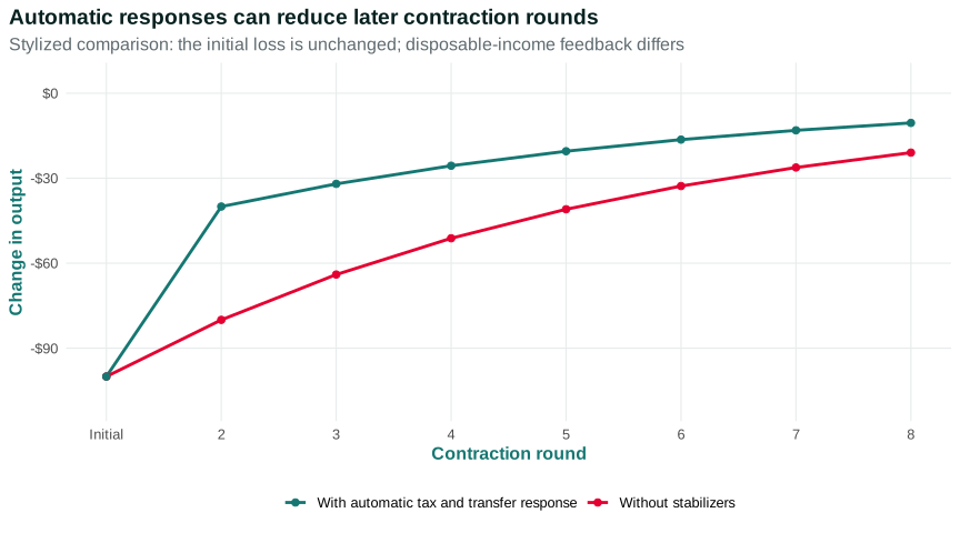
Automatic stabilizers are fiscal features that change with income and employment under existing rules, without a new legislative decision. When earnings fall, tax payments often fall. When eligible workers lose jobs, unemployment benefits and some other transfers rise. These changes cushion disposable income and can reduce the size of later spending cuts.
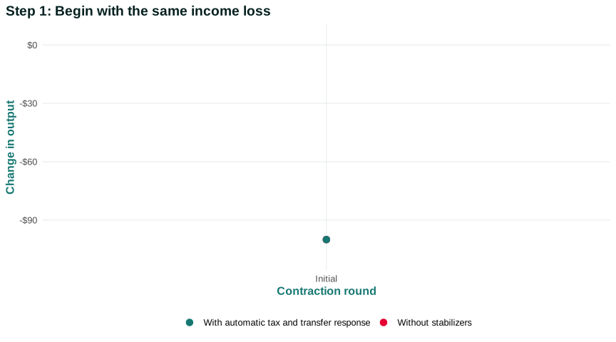
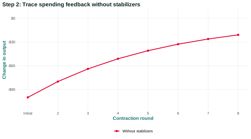
Suppose a worker loses $100 of labor income. Without taxes or transfers, disposable income falls by $100. With an automatic tax reduction of $15 and a $35 benefit payment, disposable income falls by $50. If the worker spends 80 percent of changes in disposable income, the immediate consumption cut is $40 rather than $80. The stabilizer does not erase the job loss. It changes how strongly the loss enters the next spending round and who bears it.
Figure 6.3 traces a stylized contraction with and without this cushion. The first production loss is identical. The later rounds differ because disposable income and consumption respond differently.
Open the live step-by-step figure
The figure is analytical, not an empirical estimate. Actual effects depend on eligibility, benefit amount and duration, administrative delays, tax structure, household response, state finance, and the behavior of employers and creditors. If applications are difficult or benefits arrive late, the formal rule may provide less immediate stabilization. Institutions matter through implementation, not only statutory design.
Trade and sectoral transmission
If a household spends an added dollar on an imported good, part of the income is generated abroad. Domestic distributors, retailers, and transport providers may still receive value added, so import leakage is not all-or-nothing at the product level. The domestic content of spending matters.
Exports create the reverse connection. A fall in foreign income can reduce demand for US exports and initiate a domestic contraction. Exchange rates, global supply chains, trade credit, and foreign policy responses affect the magnitude. The Interdependence principle is not an abstract claim: domestic incomes are linked to decisions made by households, firms, and governments elsewhere.
Stabilization redistributes risk
Automatic stabilizers shift some short-run income risk from households and firms toward public budgets. That can protect consumption and reduce costly eviction, hunger, debt default, or business closure. It also changes public borrowing and future fiscal choices. The incidence depends on who pays taxes, who qualifies for benefits, which governments face balanced-budget rules, and whether aid reaches places experiencing the largest shocks.
We should not say simply that “government stabilizes the economy.” Legislatures design eligibility and financing. Agencies process claims. State and local governments operate under different constraints. Courts interpret rules. Households may lack information or documentation. The strength and distribution of the response are institutional outcomes.
Discretionary fiscal policy differs from an automatic stabilizer. A legislature may enact new purchases, grants, tax changes, or transfers in response to a downturn. The action can be large and targeted, but authorization, procurement, and implementation take time. Automatic rules can respond faster once a person’s income or eligibility changes, but outdated administrative systems or narrow eligibility can delay them as well. “Automatic” describes the absence of a new legislative vote, not the absence of administrative work.
The public budget also responds to the economy. A recession can reduce tax receipts and raise transfers even with no policy change. A larger deficit is therefore partly an outcome of the contraction. Treating every deficit increase as a new discretionary stimulus reverses the direction of explanation. Chapter 12 will separate budget identities, debt stocks, financing, and sustainability claims in detail.
The next section moves from an average MPC to unequal household balance sheets. This is necessary because the same income loss can generate very different spending responses.
Questions
Question 6.4. Which is an automatic stabilizer?
- A new emergency spending law
- Unemployment benefits rising under existing rules
- A firm lowering price
- A central bank press conference
Exercise
Leakages and stabilizers
Trace how taxes, imports, and unemployment benefits alter spending-income feedback after job loss.
The model solution is available in the restricted instructor materials.
6.5 Consumption smoothing and unequal constraints
People try to separate spending from temporary income changes
People often try to smooth consumption: to prevent a temporary income change from producing an equally abrupt change in living standards. A household can draw down savings, borrow, postpone debt repayment, sell an asset, receive family support, claim insurance, or adjust hours of paid and unpaid work.
These options are not distributed equally. Consider three households that each lose $1,000 of monthly labor income.
| Household position | Liquid resources and obligations | Feasible immediate response | Likely spending sensitivity |
|---|---|---|---|
| Renter with little cash | Rent due, credit near limit, no paid leave | Cut food, transport, care, or bills quickly | High |
| Middle-wealth homeowner | Some checking savings and unused credit | Draw down cash or borrow temporarily | Moderate, but debt exposure rises |
| High-wealth household | Large liquid assets and diversified income | Maintain consumption and rebalance assets | Often lower for a small temporary loss |
The table does not claim every person in a category behaves alike. It identifies constraints. A low-income household may receive strong family or public support. A wealthy owner may face a severe business liquidity crisis. A household with retirement wealth can still lack cash. Expectations about whether the loss is temporary can outweigh the current balance sheet.
Debt repayment reveals why an individual’s prudent balance-sheet action may weaken current demand without making money disappear. If a household uses an added $500 to repay a credit-card balance, the lender receives a financial payment rather than a purchase of current goods or services. The lender can extend new credit or distribute income, but that next step is not guaranteed. The repayment can improve the household’s future interest burden while contributing little to the immediate consumption round.
This distinction is especially important after a debt-financed boom. Households may prioritize repairing balance sheets, banks may tighten standards, and firms may see few customers even when interest rates are low. The simple MPC can summarize the immediate spending response, but balance sheets help explain why the response changed. Chapters 11–13 will model borrowing, banking, leverage, and default directly.
Credit is an institution and a power relationship. Lenders decide approval, interest rates, limits, collateral, fees, and default consequences. Borrowing can smooth consumption today while moving risk into the future. A landlord or creditor may continue receiving payment because a tenant or debtor cuts other spending. Aggregate consumption is therefore built from contracts and claims, not one representative household.
Insurance and public provision alter the multiplier
Unemployment insurance replaces part of lost earnings for eligible workers. Health insurance can prevent a health shock from becoming an immediate spending collapse, though deductibles and employment-linked coverage can transmit risk. Paid leave can maintain income when care or illness interrupts work. Food assistance can protect consumption in a targeted category. These programs alter both well-being and spending feedback.
Empirical studies of unemployment and benefit exhaustion find that spending responds to cash-flow changes, including predictable benefit endings. Studies of stimulus payments also find heterogeneous and time-dependent consumption responses. Such evidence rejects the idea that all households perfectly smooth every temporary change. It does not imply that one MPC applies to every policy or period. Ganong and Noel (2019)
Class shapes these mechanisms through ownership, wage dependence, wealth, authority, and intergenerational resources. Race and gender intersect through wealth gaps, occupational exposure, discrimination in credit and housing, care responsibilities, and program access. Place matters because housing costs, public services, labor markets, and state benefit systems differ. Citizenship and disability can affect eligibility, administrative burden, and feasible work.
Aggregating heterogeneous households
Suppose half of an added $100 goes to households with an MPC of 0.9 and half to households with an MPC of 0.3. The first induced consumption round is $60: $45 from the first group plus $15 from the second. If the entire payment instead went to the high-MPC group, the first round would be $90. The distribution of an income change can affect aggregate demand even when its total dollar amount is unchanged.
This does not establish that the highest-MPC allocation is always the best policy. Policymakers may value insurance, rights, administrative feasibility, long-run investment, or poverty reduction separately from short-run output. Transfers must be financed, and supply conditions matter. The example shows only that distribution can enter the mechanism rather than being attached as an afterthought.
Household consumption is one component of aggregate demand. Firms also make forward-looking and finance-dependent spending decisions, often in large discrete amounts. We turn next to investment.
Data Extension 6.5.1: Cash flow, benefits, and spending
Researchers estimate consumption responses by finding income changes whose timing or eligibility provides a credible comparison. One study of the 2008 US stimulus payments used variation in when households received payments. The authors found substantial spending responses, but the size differed by spending category and household characteristics. Research on unemployment-insurance recipients has found that spending falls when workers lose jobs and can fall again when benefits expire. Parker and coauthors (2013)
These studies do more than calculate a correlation between income and consumption. If a household receives a payment in a month when its income was already rising for another reason, a simple before-and-after comparison would mix the two causes. A research design seeks a comparison group or timing difference that approximates what the recipient would have spent without the income change.
| Feature | Question |
|---|---|
| Income change | Was it expected, temporary, persistent, cash-like, or restricted? |
| Population | Which households were observed, and who was excluded? |
| Spending measure | Nondurables, durables, total outflows, or a specific merchant category? |
| Time horizon | Immediate weeks, a quarter, or a year? |
| Identification | What creates the comparison used for a causal claim? |
The resulting number should not be copied directly into every multiplier exercise. A household MPC out of one payment is not the same as the total output effect of a government program. The latter also depends on financing, imports, firms’ production responses, prices, monetary policy, and further rounds. Micro evidence informs one behavioral link inside the aggregate mechanism.
Use Parker and coauthors’ stimulus-payment study or Ganong and Noel’s unemployment-spending study to identify the population, income change, spending outcome, and comparison strategy. Then explain one reason the estimate may differ for another group or recession.
Questions: Why is randomized payment timing useful? Why would spending at benefit exhaustion be relevant to automatic stabilization? Which additional steps are required before calling either estimate a fiscal multiplier?Questions
Question 6.5. Who is most likely to cut spending quickly after income loss?
- A household with little liquid saving and no credit
- A household with ample liquid wealth
- Every household equally
- Only firms
Exercise
Capacity to smooth
Compare the options of two households with equal income loss but different savings, debt, and family support.
The model solution is available in the restricted instructor materials.
6.6 Investment and expectations
Firms compare future revenue with current commitment
Investment includes business fixed investment, residential construction, and inventory accumulation in the national accounts. Buying an existing share or bond is a financial transaction; building a new warehouse or installing new equipment is current investment production.
A firm considering a new machine asks whether future sales will justify its purchase, installation, training, maintenance, and financing costs. The decision depends on expected demand, the machine’s productivity, interest and credit terms, existing capacity, uncertainty, and how easily the decision can be reversed.
| Changed condition | Effect on the firm’s decision problem | Possible investment response |
|---|---|---|
| Expected future sales fall | The machine is less likely to be fully used | Delay or cancel |
| Borrowing cost rises | More future revenue is needed to cover finance | Reduce or redesign project |
| Credit line is withdrawn | A profitable project may become infeasible | Cancel despite expected demand |
| Existing capacity is nearly full | Lost sales from delay become more likely | Accelerate investment |
| Public infrastructure improves | Private production may become more productive | Expand complementary investment |
Expectations can amplify a downturn. Weak current sales lead firms to expect weak future sales. They cut investment. The investment cut reduces current orders and income, which can make weak future sales more likely. This is an aggregation feedback, not proof that pessimism alone causes recessions. Expectations may be responding accurately to public health, financial fragility, technology, or policy.
Figure 6.4 separates the decision from the feedback. Step 1 begins with a firm’s expected sales and financing constraint. Step 2 adds the investment choice. Step 3 traces how lower investment reduces income and realized sales, feeding back into later expectations.
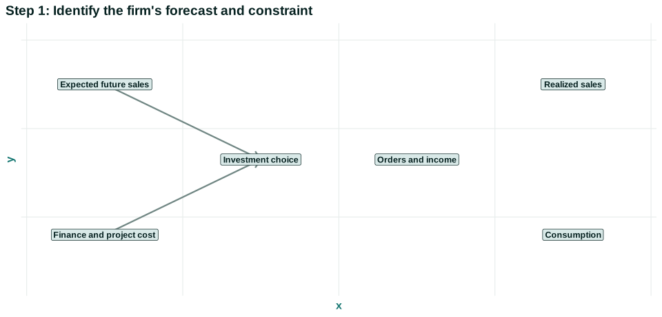
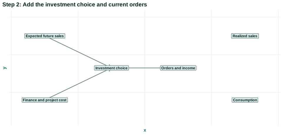
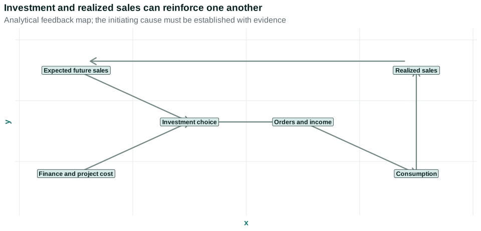
Open the live step-by-step figure
Finance gives some actors authority over the feasible set. Bank lending standards, collateral values, bond-market access, and internal cash determine which firms can act on an opportunity. Large firms may issue securities while a small local business relies on one bank or personal collateral. A decline in asset values can therefore reduce investment even if the project’s technology has not changed.
Investment can also lead a recovery. Public purchases, household demand, new technology, or improved expectations raise desired capacity. New orders become income for equipment producers and construction workers, creating multiplier rounds. But if the economy is already using its capacity intensively, additional demand can produce delivery delays and price pressure rather than proportionate real output. Chapter 8 returns to those supply and price limits.
The investment relationship is behavioral and forward-looking. An observed correlation between investment and GDP does not identify a one-way causal effect because current income, expectations, finance, and investment influence one another. Research designs must find changes in investment or spending not caused by the same factors simultaneously moving output.
Housing investment makes the feedback concrete. Builders respond to expected sale prices, mortgage demand, land rules, material costs, and finance. A fall in home demand can reduce construction employment and purchases of appliances and materials. Falling local incomes can then weaken housing demand further. Yet supply restrictions can also keep prices high while construction remains limited. “Investment fell” is an accounting description; explaining it requires the specific market and institutions.
Inventory investment can move in the opposite direction from firms’ intentions. If sales disappoint, unsold goods raise measured inventory investment in the current accounts even while managers plan to cut future production. A high recorded investment number is therefore not always evidence of optimism. Students should ask whether inventory accumulation was planned and how firms responded afterward.
We end with the clearest example of why individually sensible choices do not simply add up: the paradox of thrift.
Questions
Question 6.6. Why can investment amplify a downturn?
- Expected weak sales can reduce investment and income
- Investment is fixed by identity
- Firms never use credit
- Inventories are excluded from GDP
Exercise
Expectations feedback
Construct a causal chain from expected weak sales to investment, income, and realized sales; name evidence needed to test it.
The model solution is available in the restricted instructor materials.
6.7 The paradox of thrift and the limits of the model
A prudent choice can change the environment in which everyone chooses
Saving more can strengthen one household’s balance sheet. It can provide emergency funds, reduce debt, finance education, or support retirement. Nothing in the multiplier model says an individual household is foolish to save.
Now suppose many households simultaneously try to raise saving by cutting consumption. Firms receive fewer orders. With spare capacity and fixed prices, they reduce production and income. Lower income induces further consumption cuts. Because total saving depends on both the fraction of income saved and the level of income, realized aggregate saving may rise by less than households intended—or not rise at all.
The paradox of thrift is this possibility that simultaneous attempts to save more reduce aggregate demand and income enough to frustrate the aggregate saving goal. It is a result about feedback, not a condemnation of thrift.
Trace the logic with numbers. Initially, households receive $1,000 of income, consume $800, and save $200. They attempt to save $250 by cutting consumption to $750. That $50 spending reduction lowers other people’s income. With a multiplier of 2, equilibrium income falls by $100. If the new economy-wide propensity to consume produces $720 of consumption from $900 of income, realized saving is still $180—lower than before. The exact result depends on behavior and investment; the example shows why the intended dollar saving cannot be calculated while holding aggregate income fixed.
This is the Principle of individual and societal interests. Each household responds to its own risk. The combined response changes sales, employment, and income, altering every household’s choice environment. It is also the Principle of aggregation and feedback: the aggregate outcome is not a simple sum of plans because plans affect one another through income.
Saving can finance investment—but the link is not automatic
In a longer-run and financial perspective, saving can provide funds for investment. But a household’s additional bank balance does not guarantee that a firm wants to borrow and invest during a slump. Banks may tighten lending, firms may expect weak demand, and the central bank may change interest rates. The paradox concerns a demand-constrained short run in which intended saving rises without an offsetting rise in investment or another spending component.
If firms become more optimistic and raise investment by the amount households cut consumption, aggregate demand need not fall. If government purchases rise, exports increase, or automatic stabilizers support disposable income, the contraction can be smaller. Naming what is held fixed is essential.
What the multiplier model leaves out
The simple model assumes that firms can expand production at given prices. That may be reasonable in a deep recession with idle workers and equipment. It becomes less reasonable near capacity or during a supply disruption. Additional spending may then raise prices, imports, overtime, or delivery delays rather than real output in the same proportion.
The model also omits monetary policy. Interest-rate changes affect borrowing, asset prices, exchange rates, housing, and investment. If a central bank offsets fiscal expansion, the observed multiplier differs from a case in which monetary policy accommodates it. Financial distress, default, and bank balance sheets can create additional feedback. Expectations may change before spending occurs.
Empirical multipliers therefore vary by policy, recipients, timing, openness, economic slack, monetary response, and research design. A number estimated from one historical episode is not a universal constant. The classroom multiplier is valuable because it identifies a mechanism and its assumptions; evidence is required to measure its strength in a particular setting.
Researchers face a difficult counterfactual. Governments often increase spending when the economy is already weakening, while tax revenue automatically falls. A simple comparison between high spending and low output might therefore suggest that spending reduces output even when policy cushioned a larger decline. Alternatively, an anticipated program can change household and firm behavior before the first recorded expenditure. Identifying a causal multiplier requires a source of policy variation, a time horizon, and a statement of what other policies did.
Composition matters as much as the headline amount. A construction project purchases labor and materials directly but may take time to begin. A transfer can arrive quickly but generates demand according to recipient behavior. Aid to a state government may prevent layoffs rather than create a new visible project. A tax change can alter take-home pay, incentives, or balance sheets. Calling all of these “a dollar of stimulus” erases the mechanism the estimate is supposed to measure.
When unemployment is high and equipment is idle, firms may meet higher demand by expanding real production. Near capacity, more adjustment may occur through prices, imports, or monetary tightening. Historical episodes differ in many dimensions at once, so estimates of how multipliers vary with economic slack are contested. The safe lesson for this chapter is conditionality, not one preferred numerical range.
Finally, higher aggregate demand does not distribute benefits or costs equally. Workers in expanding sectors may gain hours and bargaining power. Owners may receive profits. Renters may face price increases if housing supply is tight. Taxpayers and beneficiaries occupy different positions. Public debt changes future claims but does not mechanically impose one equal burden on every person. Distribution belongs inside policy analysis.
Chapter 5 taught us to keep accounting identities separate from causal claims. Chapter 6 has added a behavioral relationship and followed its feedback. Later chapters add inflation, supply constraints, monetary policy, fiscal institutions, finance, and the international economy. The multiplier is the beginning of aggregate-demand reasoning, not a complete macroeconomic theory.
Seeing the principles in action
| Principle | Example | Everyday Economics |
|---|---|---|
| Interdependence principle — focal | One person’s spending becomes another person’s income across households, firms, government, and trade. | A cancelled restaurant meal affects workers and suppliers. |
| Doing the best you can principle | Households smooth consumption and firms invest given wealth, credit, risk, and expectations. | A household without savings cuts spending faster after job loss. |
| Rules of the game principle | Taxes, transfers, unemployment insurance, and credit rules change how shocks pass into disposable income. | An automatic benefit payment cushions a lost paycheck. |
| Trade-offs and opportunity costs principle | Spending now gives up saving; restraint now can also reduce another person’s income. | Postponing a purchase preserves cash but reduces a seller’s revenue. |
| Principle of gains from cooperation and conflict of interest | Coordinated recovery can raise income, while conflict concerns who finances support and who receives it. | A local recovery plan can help shops and workers but distribute costs unevenly. |
| Principle of individual and societal interests — focal | Individually prudent saving can reduce aggregate income when many people do it together. | Every family can intend to save more even if total saving fails to rise. |
| Principle of aggregation and feedback — focal | The multiplier is repeated feedback from spending to income to further spending. | A first lost sale can generate later lost sales. |
Skills and learning objectives
- Tracing spending-income feedback
- Distinguishing behavior from accounting
- Calculating a simple multiplier
- Evaluating unequal consumption responses
- Explaining the paradox of thrift
Concepts to learn
- Aggregate demand
- Marginal propensity to consume
- Multiplier
- Automatic stabilizers
- Consumption smoothing and credit constraints
- Investment and expectations
- Paradox of thrift
Glossary
Chapter 6 terms
aggregate demand
Total planned spending on domestically produced goods and services under stated economic conditions.
See also: multiplier.
marginal propensity to consume
The fraction of an additional dollar of disposable income spent on consumption in the model.
See also: multiplier; consumption smoothing.
multiplier
The total change in equilibrium output divided by the initial change in autonomous spending that set off repeated income-spending feedback.
See also: marginal propensity to consume; aggregate demand.
leakage
Income not passed into the next round of domestic consumption in a multiplier sequence, including saving, taxes, and spending on imports under the model’s stated conditions.
See also: multiplier; marginal propensity to consume.
automatic stabilizers
Taxes and transfers that change with income and employment without a new legislative decision, moderating fluctuations in disposable income and demand.
consumption smoothing
Using saving, borrowing, insurance, or other resources to keep consumption from moving one-for-one with temporary income changes.
See also: marginal propensity to consume.
investment
Spending on new capital goods, residential structures, and inventory accumulation under the national accounts definition.
paradox of thrift
The possibility that simultaneous attempts to save more reduce aggregate demand and income enough that total saving does not rise as intended.
See also: multiplier.
Flashcards
What is the marginal propensity to consume?
The share of an additional dollar of disposable income spent on consumption in the model.
What creates the multiplier?
Repeated feedback in which one actor’s spending becomes another’s income and supports further spending.
What is the paradox of thrift?
Simultaneous attempts to save more can reduce income enough that aggregate saving does not rise as intended.
Questions
Question 6.7. The paradox of thrift concerns…
- one household saving for an emergency
- simultaneous saving attempts reducing aggregate income
- government always borrowing
- imports always exceeding exports
Exercise
Paradox of thrift
Explain how every household can intend to save more while aggregate saving fails to rise, and state one model limitation.
The model solution is available in the restricted instructor materials.