Fiscal Policy: Spending, Taxes, Transfers, Deficits, and Debt

Works Progress Administration project in Cambria, Illinois, 1939. Arthur Rothstein, Farm Security Administration, Library of Congress. View the Library of Congress record. No known restrictions.

Public working draft: This AI-assisted feasibility draft is open for coauthor revision. Empirical descriptions, causal claims, program details, debt analysis, and figure rights remain subject to human review.

Central question: When the economy is hit by a shock, how do fiscal institutions change spending, share risk, and distribute the costs—and what limits their response?

By the end of this chapter, you should be able to: distinguish purchases, transfers, taxes, and financial transactions; explain how automatic stabilizers cushion disposable income; trace discretionary fiscal policy through demand and production; identify conditions that change a fiscal multiplier; distinguish a deficit flow from public debt; explain why federal and state governments face different constraints; and evaluate a fiscal package by its goal, timing, implementation, distribution, and financing.

9.1 The same shock, different fiscal positions

In April 2020, imagine two budget meetings. At one kitchen table, a worker whose hours disappeared checks a bank account for a federal payment and tries to decide which bills can still be paid. At a city budget office, officials see transit fares, sales-tax receipts, and other revenue collapse while residents need more public help. Both meetings concern spending during the same emergency. Yet the household, the federal government, and the city do not have the same authority or financing options.

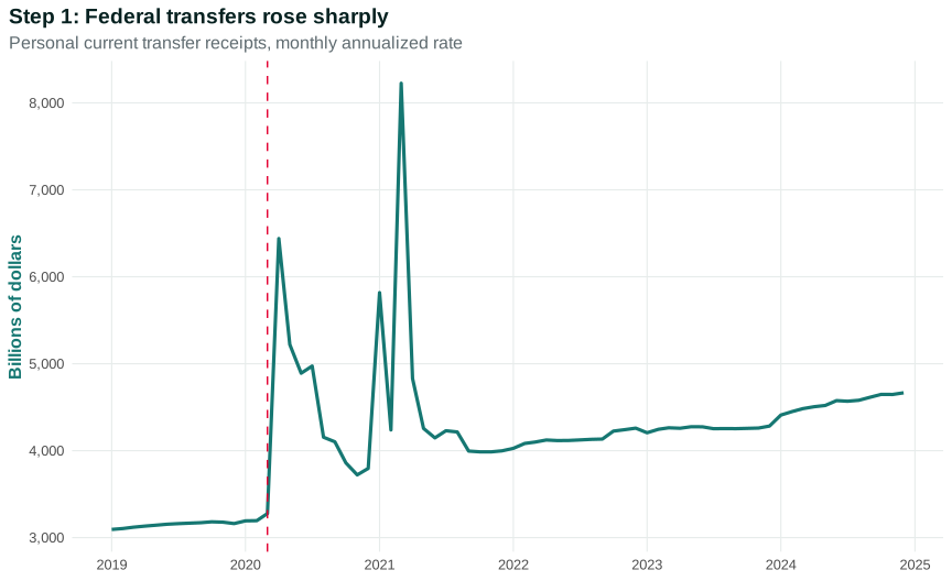
Figure 9.1 begins with personal current transfer receipts. This national BEA measure includes far more than pandemic relief, and it is shown at an annualized monthly rate. A value of $6 trillion does not mean households received $6 trillion in that month. It means that month’s pace multiplied by twelve would equal $6 trillion. The spike is therefore evidence about timing and scale, not a payment total.

Step 1: Federal transfers

Federal personal current transfer receipts rise sharply in 2020.

Step 2: State and local employment

State and local government employment falls sharply in 2020.

Summary figure

Figure 9.1: Federal transfers and state/local employment during the pandemic shock. Sources: BEA and BLS via FRED.

Open the live step-by-step figure

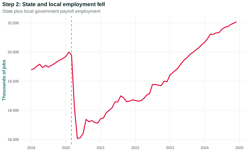
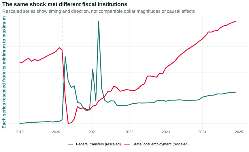
The second step adds combined state and local government employment. It is measured in thousands of payroll jobs, not dollars. The summary rescales each series between its own lowest and highest value only so we can compare direction and timing. A rescaled value of one for transfers is not comparable in magnitude to one for employment.

The pattern is memorable: federal transfers rose while subnational public employment fell. But the figure cannot tell us how much transfers changed household spending, whether the fall in public employment was caused by revenue rules rather than closures or health risks, or what would have happened without policy. Those are causal questions requiring comparisons and institutional evidence.

The contrast does identify a mechanism worth explaining. The federal government can borrow in national financial markets and create transfers through federal law. Most state and local governments operate under balanced-budget requirements and cannot issue currency. Their revenues can fall precisely when demands on services rise. Federal grants can relax that constraint, but only if legislation, allocation rules, and administration deliver resources in time.

This chapter therefore follows three sets of actors. Households want to meet needs and manage uncertainty. Governments want to provide services, stabilize the economy, and satisfy legal and political commitments. Taxpayers, public employees, benefit recipients, contractors, and creditors have different interests in the instruments chosen. When a shock arrives, how do fiscal institutions change spending, share risk, and distribute the costs—and what limits their response?

Questions

Review the live step-by-step figure

Question 9.1. What is the strongest conclusion from Figure 9.1?

1. Federal transfers rose while state/local employment fell during the same shock
2. Transfers caused every employment change
3. The two series have the same units
4. State governments can borrow exactly like the federal government

Exercise

Two fiscal positions

Use Figure 9.1 to state one descriptive pattern, one institutional hypothesis, and one causal claim the figure cannot establish.

The model solution is available in the restricted instructor materials.

9.2 What fiscal policy can change

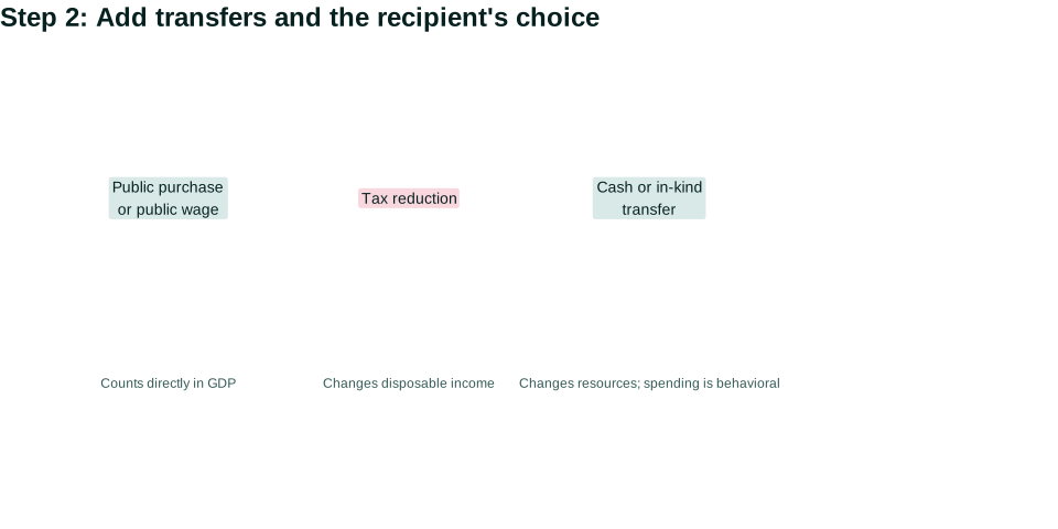
Fiscal policy means government decisions and rules concerning purchases, public employment, taxes, transfers, and borrowing. The label becomes useful only after we distinguish the transactions. A city buying buses, the federal government sending a benefit payment, and a public agency making a loan can all appear in a news story as “government spending,” but they enter national accounts and household decisions differently.

A government purchase pays for currently produced goods or services: a teacher’s labor, a vaccine, a bridge inspection, or computer equipment. It enters GDP directly because the government is a buyer of current production. A transfer changes who can spend without purchasing current production in that transaction. Social Security, unemployment insurance, and a cash relief payment therefore do not enter GDP directly. They can affect GDP when recipients alter consumption.

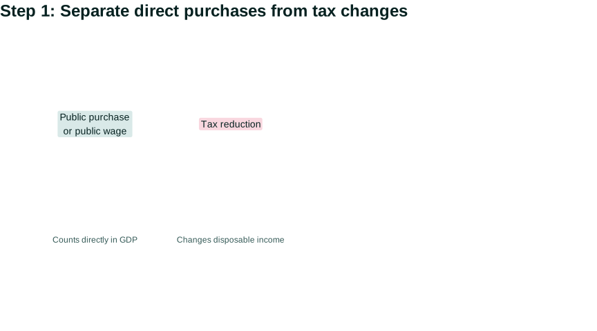
A tax changes the resources an actor can use, incentives, and sometimes prices. If a household’s pretax income is $4,000, taxes are $600, and cash benefits are $300, its disposable income is $3,700. Reducing taxes by $200 or increasing the cash benefit by $200 produces the same immediate arithmetic. It need not produce the same behavior: eligibility, timing, permanence, debt, liquidity, and who receives the change differ.

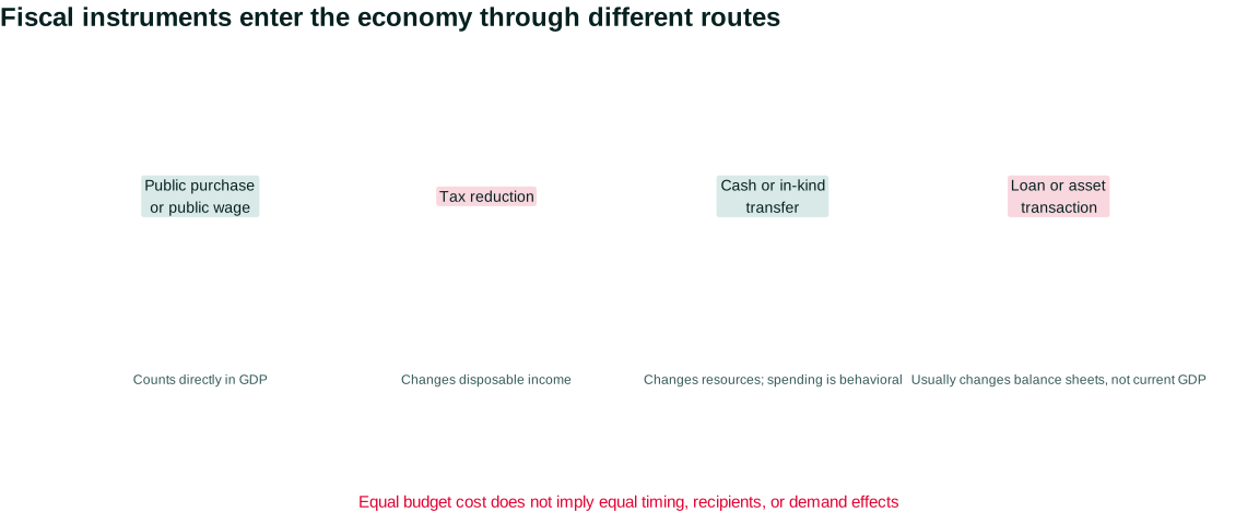
Figure 9.2 keeps accounting and behavior separate.

Step 1: Purchases and taxes

Public purchases enter GDP directly while taxes change disposable income.

Step 2: Add transfers

Transfers change resources and recipients then decide how much to spend.

Summary figure

Figure 9.2: Four fiscal transaction types and their routes into the economy.

Open the live step-by-step figure

A loan is different again. If a government lends $10,000 to a small business and receives a promise of repayment, both sides change their balance sheets. The transaction is not itself $10,000 of current production. If the business then buys equipment or pays workers to produce goods, those later transactions can enter GDP. Loan guarantees can change credit availability even when little cash is initially spent.

These distinctions stop two common mistakes. First, a headline budget cost is not the same as a contribution to GDP. Second, an equal budget cost does not imply an equal effect on demand. A $1 billion purchase creates $1 billion of direct demand for specified production, though delivery may take time. A $1 billion transfer changes recipient resources; some may be spent quickly, some used to repay debt, and some saved. Repaying debt can still protect a household and reduce default risk, even if its immediate demand effect is smaller.

The distinctions also clarify the national-income identity. Government purchases appear in the expenditure measure of GDP. Taxes and transfers do not appear there as separate additions or subtractions, although they change disposable income and behavior. This is an accounting statement about how transactions are recorded, not a claim that taxes and transfers are economically unimportant. If a transfer enables a grocery purchase, the consumption appears when the purchase occurs. If the transfer prevents an eviction or allows debt repayment, that benefit may matter even though the transaction does not add directly to current GDP.

Follow the actors rather than the budget label. A legislature authorizes an instrument. An agency translates authority into eligibility, contracts, or payment systems. A household, public employer, contractor, lender, or seller then adjusts. Firms respond to sales and capacity; workers respond to jobs and income; tax receipts and benefit claims may respond again. Fiscal policy is therefore both an accounting change and a chain of institutional and behavioral responses.

Fiscal policy also changes supply and public capacity. Childcare can allow more caregivers to take paid work. Public health can prevent production losses. Infrastructure can increase later productivity. Conversely, poorly designed procurement can waste resources or crowd out urgent private uses when the economy is at capacity. Short-run stabilization is only one goal of public action.

The next question is whether fiscal policy always requires a new vote. Many tax and benefit rules respond automatically as income and employment change.

Questions

Review the live step-by-step figure

Question 9.2. Which transaction enters GDP directly?

1. A cash transfer
2. A government purchase of current services
3. A tax refund by itself
4. A government loan disbursement by itself

Exercise

Classify transactions

Classify a school wage, unemployment benefit, tax rebate, and public loan by direct GDP entry and behavioral route.

The model solution is available in the restricted instructor materials.

9.3 Automatic stabilizers

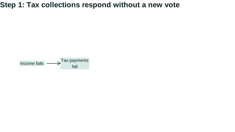
An automatic stabilizer is a tax or spending rule that changes with economic conditions without new discretionary legislation. When earnings fall, income-tax payments usually fall. When eligible workers lose jobs, unemployment-insurance payments rise. During an expansion, the directions reverse. CBO calls these automatic because existing law makes revenues and outlays respond to cyclical changes, not because administration happens instantly or without choices. CBO automatic-stabilizer definition

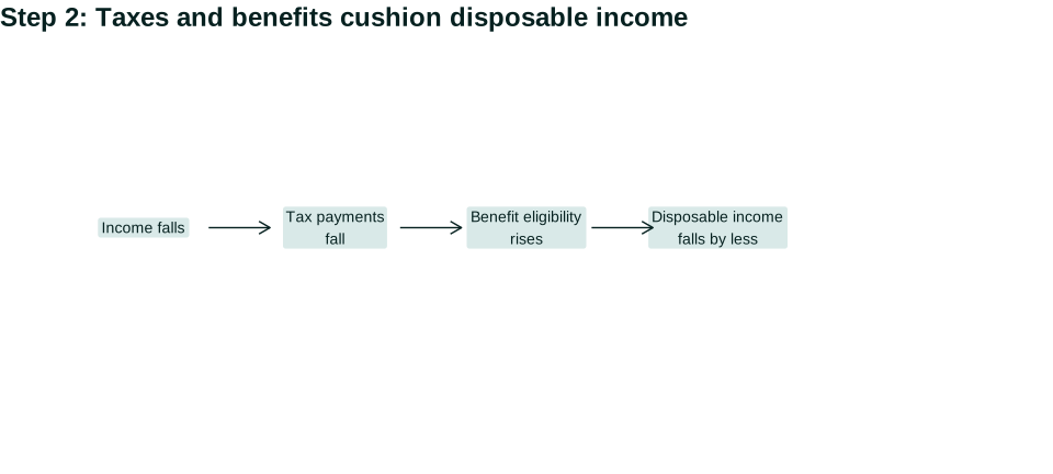
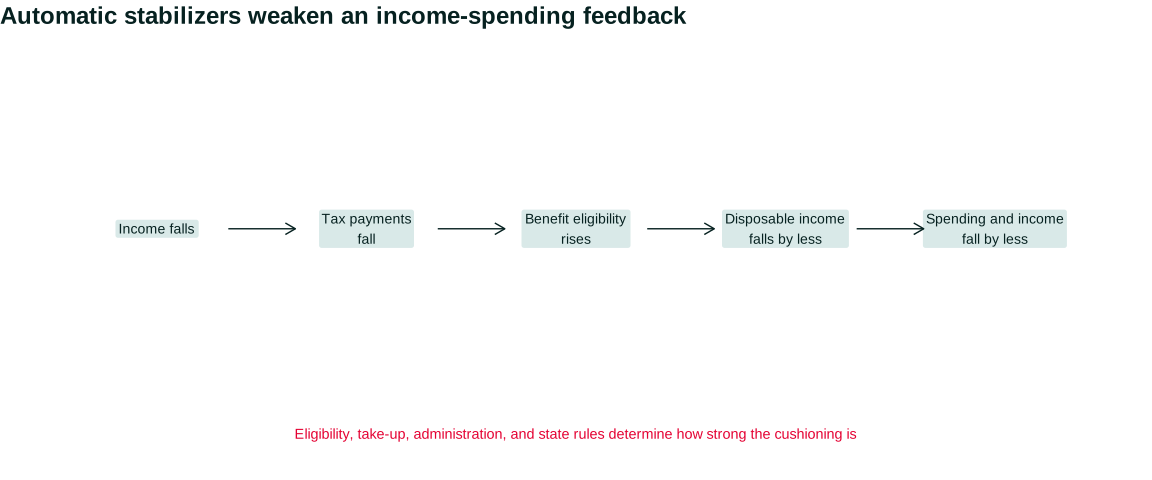
Take a simple household. Monthly market income falls from $4,000 to $2,000. Under an assumed 20 percent tax, taxes fall from $800 to $400. Suppose the household also qualifies for $600 in benefits. Disposable income falls from $3,200 to $2,200—by $1,000 rather than the full $2,000 market-income loss. The rule cushions half the shock in this example.

Monthly situation	Market income	Tax	Benefit	Disposable income
Before job loss	$4,000	$800	$0	$3,200
After, taxes only adjust	$2,000	$400	$0	$1,600
After, taxes and benefit adjust	$2,000	$400	$600	$2,200

The numbers are assumptions, not descriptions of one actual program. Real tax schedules have deductions, credits, payroll taxes, filing lags, and family rules. Unemployment insurance varies by state, prior earnings, work history, reason for separation, immigration status, application success, and benefit duration. Eligibility is not the same as receipt.

Figure 9.3 shows the feedback that the arithmetic interrupts.

Step 1: Taxes respond

Lower income produces lower tax payments under existing rules.

Step 2: Benefits cushion disposable income

Lower taxes and higher benefit eligibility reduce the fall in disposable income.

Summary figure

Figure 9.3: Automatic stabilizers weaken the income-spending feedback.

Open the live step-by-step figure

If households spend part of each additional dollar of disposable income, cushioning their income cushions someone else’s sales and income. This is the Aggregation and feedback principle. The stabilizer does not prevent every decline. It weakens one feedback loop.

Design determines both stabilization and distribution. A progressive tax responds more strongly to income changes near the top, while refundable credits can support low-income households. Benefits directed to people with little liquidity may be spent quickly because urgent needs were already unmet. Administrative delays, exclusions, digital access, documentation, and stigma can weaken the response. Rules reflect political authority as well as technical design.

Automatic stabilizers also change the budget balance. In a downturn, revenues fall and some outlays rise even if lawmakers pass no bill. A larger deficit is therefore partly an effect of the downturn. Treating every deficit increase as evidence of a new discretionary expansion reverses the direction of causation.

This distinction is visible in CBO’s historical estimates. Over 1974–2023, CBO estimates that automatic stabilizers increased federal deficits by an average of 0.4 percent of potential GDP per year. That average does not describe every recession, and it does not measure the total effect of fiscal policy. It shows that part of the observed budget balance moves with the economy under existing law. To judge a new bill, we must separate that automatic response from the discretionary change. CBO historical automatic-stabilizer estimates

The word automatic can therefore mislead in two directions. It does not mean benefits arrive without applications, records, staffing, or appeals. It also does not mean legislators have surrendered authority: lawmakers designed the formulas and can change them. Automatic stabilizers are rules chosen in advance, implemented by institutions, and experienced by people whose access differs.

Rules provide speed, but an unusual shock may exceed what existing programs cover. That creates the case for discretionary policy.

Questions

Review the live step-by-step figure

Question 9.3. An automatic stabilizer is…

1. a rule that responds to conditions without new legislation
2. every emergency spending bill
3. a promise that income never falls
4. a fixed multiplier

Exercise

Cushioning arithmetic

Change the assumed tax rate and benefit in the Section 9.3 table and calculate the fraction of market-income loss cushioned.

The model solution is available in the restricted instructor materials.

9.4 Discretionary fiscal policy

Discretionary fiscal policy requires a new legislative or administrative decision. Lawmakers can authorize purchases, aid to state governments, transfers, tax changes, credit support, or public investment. The relevant question is not simply whether the package is “large.” It is whether the instrument matches the problem.

Relief, recovery, and investment have different goals. Relief helps people meet needs and preserves relationships during a temporary disruption. Recovery policy raises demand when idle labor and capacity can respond. Public investment aims to expand capacity or improve services over a longer horizon. One program can serve more than one goal, but evaluation should not silently switch criteria. A transfer may be excellent insurance even if recipients save much of it; a slowly built rail project may improve capacity even if it arrives too late to stop a short recession.

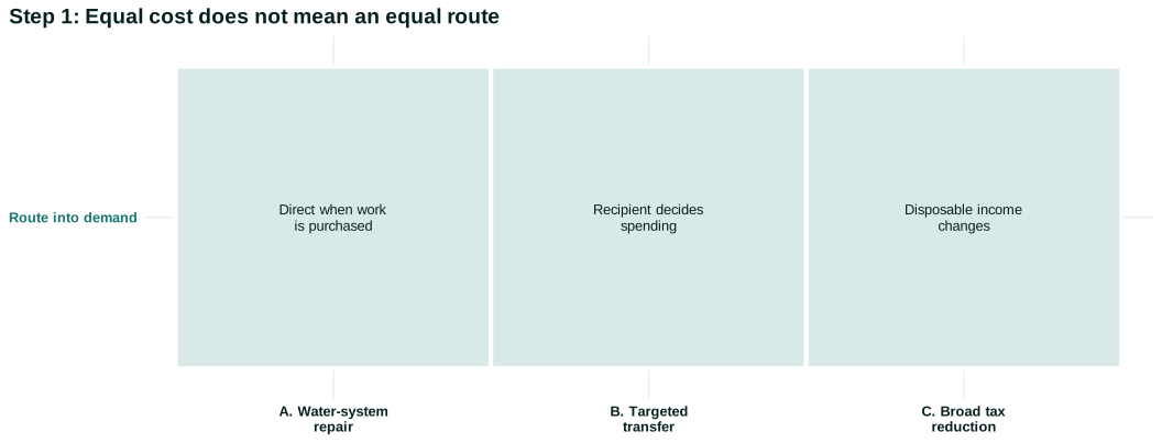
Consider three packages with the same $1 billion headline cost. The government could purchase immediate repair work, send transfers to households with recent income losses, or cut a broadly based tax. The purchase has a direct demand route but depends on project readiness, inputs, and public capacity. The targeted transfer relies on recipient spending but can reach urgent needs. A broad tax cut may be administered quickly through withholding, yet some resources go to households likely to save. There is no ranking that ignores the shock and goal.

Timing has several parts. Recognition takes time: data are revised and causes disputed. Legislation takes time: coalitions bargain over size and distribution. Implementation takes time: agencies write rules, process claims, hire staff, and procure goods. Effects then unfold with behavioral and production lags. A rule enacted quickly can still reach people slowly.

Targeting creates another trade-off. Narrow eligibility can direct funds toward high-need recipients and reduce fiscal cost, but it demands information, creates boundaries, and can exclude eligible people. Universal payments are simple and visible but allocate money to households with very different needs. Phase-outs change marginal tax rates and can create delays. “Targeted” is not automatically precise.

Incidence asks who ultimately gains or pays. A payroll tax cut is legally assigned to a worker or employer, but wages and employment may adjust. Rent relief can benefit tenants, landlords, or lenders depending on bargaining and contracts. A subsidy to a constrained industry can preserve jobs, profits, or both. Legal destination is not the same as economic incidence.

Policy also has an opportunity cost when real resources are scarce. If construction labor and materials are fully employed, a public project can bid resources away from private uses or raise prices. If workers and equipment are idle, the project can increase production. The same appropriation therefore has different effects across conditions.

A worked package comparison

Suppose a regional recession has left hotel workers unemployed, restaurants operating below capacity, and a damaged water system that must be repaired. Congress considers three $600 million packages. Package A hires contractors to repair the system. Package B sends $1,200 to 500,000 households that recently lost earnings. Package C reduces federal income-tax withholding across the region by a total of $600 million.

Begin with Package A. The appropriation does not create demand until agencies sign contracts and contractors pay for labor and inputs. If engineering plans already exist and unemployed construction workers have appropriate skills, production can begin quickly. If specialized pipe is scarce or procurement is contested, spending may be delayed. The repair produces a public service whose value is not fully measured by its short-run multiplier: safer water affects health, school attendance, business operation, and future maintenance cost.

Package B can arrive faster if the government has accurate payment information. A household behind on rent may spend the payment immediately. Another may repay a credit-card balance; that reduces default risk and future interest cost but creates less current demand. A third may save because the duration of unemployment is unknown. The average response therefore depends on the distribution of constraints, not on a psychological constant shared by all households.

Package C may be administratively simple for workers already receiving paychecks. But newly unemployed workers may have little withholding to reduce. A broad reduction also directs more dollars toward people with larger taxable earnings. The package can still affect demand and incentives, yet its reach differs from the stated regional problem. Tax administration is part of targeting.

Now change one condition. Suppose the water-repair labor and pipe are already fully employed elsewhere. Package A is more likely to raise prices or displace another project. Suppose instead that the payment system lacks current bank information. Package B arrives by mailed check after several months. Suppose payroll processors can change withholding immediately. Package C becomes fastest. The ranking changes because capacity and implementation change, not because the accounting identities changed.

Finally ask who has authority. Congress authorizes federal funds; an agency writes rules; state or local entities may select projects; contractors hire; households decide how to use transfers; courts can review disputes. Each handoff creates information, delay, discretion, and possibilities for exclusion. “Government chose $600 million” compresses a chain of actors.

This comparison is deliberately neutral about the best package. A defensible recommendation must state the goal. If urgent consumption insurance is primary, Package B may dominate despite some saving. If the water system creates severe health risk, Package A may dominate even with a slow multiplier. If rapid broad support to employed households is the goal, Package C has a plausible route. Policy evaluation begins by refusing to use one outcome as the criterion for every instrument.

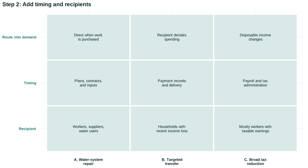
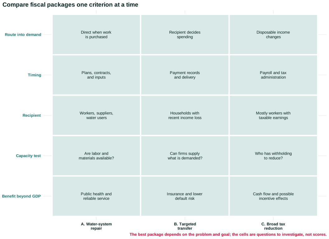
Figure 9.4 organizes the comparison. The first step holds the headline cost fixed and asks how each instrument enters the economy. The second adds the recipient and implementation constraint. Only the final step adds the public benefit and capacity question. This ordering prevents a familiar error: deciding that one package is “larger” merely because its direct route into measured GDP is larger.

Step 1: Hold budget cost fixed

Three equal-cost packages enter current spending through different routes.

Step 2: Add recipients and implementation

Recipients, administrative routes, and likely delays differ across the three packages.

Summary figure

Figure 9.4: An equal-cost fiscal package comparison across route, timing, recipient, capacity, and public benefit.

Open the live step-by-step figure

Read across a row before reading down a column. Package A enters demand directly when the purchase occurs, but it can be slow if plans or inputs are missing. Package B can reach constrained households quickly, but its effect on production depends on what recipients do and what firms can supply. Package C can change paychecks rapidly for employed workers, but it may miss people with no withholding. Now read down a column: timing, distribution, and capacity are separate criteria. A package can perform well on one and poorly on another.

To compare packages, we need a disciplined account of amplification rather than one universal number.

Questions

Question 9.4. Equal budget costs imply…

1. equal demand effects in every economy
2. equal distribution
3. nothing by themselves about equal timing or multipliers
4. that transfers count directly in GDP

Exercise

Match goal to instrument

Compare a public purchase, targeted transfer, and broad tax cut for relief, speed, distribution, and capacity.

The model solution is available in the restricted instructor materials.

9.5 How large is the fiscal multiplier?

The fiscal multiplier compares a change in output with the policy-induced change in fiscal spending or revenue under stated conditions. If a $10 billion purchase causes output to be $15 billion higher than it otherwise would have been over a specified period, the estimated multiplier is 1.5. The counterfactual phrase matters: dividing an observed GDP change by an observed budget change is not enough. TE 2.0 fiscal-policy sequence

Chapter 6 showed the feedback. Government buys services; the supplier pays workers and owners; recipients spend some additional income; other firms receive sales; imports, taxes, debt repayment, saving, and capacity limits weaken the chain. That mechanism explains why a multiplier can exceed the direct purchase. It does not guarantee a particular value.

Several conditions change the result:

• Slack: with unemployed labor and idle equipment, demand can raise quantities. Near capacity, prices, imports, and displacement may respond more.
• Recipient liquidity: a household unable to borrow against future income may spend a larger share of an immediate transfer than a buffered household.
• Persistence and expectations: a credible temporary payment and a permanent tax change can produce different plans; uncertainty can encourage precautionary saving.
• Monetary conditions: if the central bank raises rates in response to expansion, interest-sensitive spending can offset some fiscal demand. At an effective lower bound or during crisis accommodation, offset may be weaker.
• Openness: spending on imports becomes foreign rather than domestic income, though trading partners’ responses can feed back.
• Implementation and composition: purchases of available local services differ from delayed procurement of scarce imported equipment.

Crowding out is one conditional mechanism, not a slogan. Government borrowing can raise some interest rates or compete for resources. But when private investment is depressed and monetary policy keeps short rates low, public demand can raise expected sales and encourage private investment. We must specify which resource or financial channel is crowded out, when, and for whom.

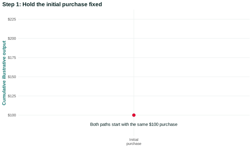
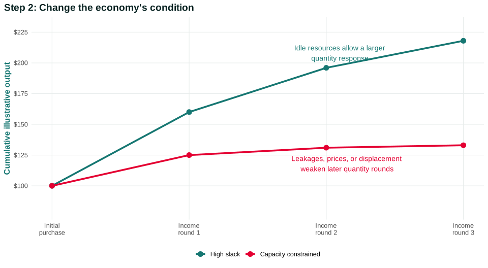
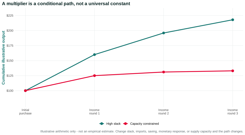
Figure 9.5 uses a deliberately simplified numerical example. Both paths begin with the same $100 public purchase. In the high-slack case, firms can respond mostly by increasing production, and each income round generates substantial additional spending. In the capacity-constrained case, imports, saving, price increases, and displacement weaken the domestic quantity response. The figure is not an estimate. It teaches why the phrase “the multiplier” is incomplete without the conditions.

Step 1: The same initial purchase

Both illustrative multiplier paths begin with the same one-hundred-dollar public purchase.

Step 2: Change the economy’s condition

Additional production rises more in the high-slack example than in the capacity-constrained example.

Summary figure

Figure 9.5: Stylized cumulative output paths under high slack and a capacity constraint.

Open the live step-by-step figure

Compare the named points after round two. The high-slack path reaches $160 of cumulative output in the illustration; the capacity-constrained path reaches $125. Nothing about the original $100 appropriation changed. What changed was the response of production and spending. If imports rose in the first path, or if the central bank raised rates, the paths would move closer. If public spending relieved a bottleneck, the capacity-constrained path could improve over time.

Causal estimates vary because policies, populations, periods, and methods vary. A transfer timed by administrative rules can support a different research design from a nationwide infrastructure law. A local military-procurement estimate may not include national monetary or tax responses. A wartime multiplier may not apply to a pandemic. Honest synthesis explains heterogeneity rather than averaging everything into a timeless constant.

Federal Reserve researchers comparing different phases of the US business cycle find that conclusions about state-dependent multipliers depend on how the state of the cycle is defined. In their estimates, rising rather than simply high unemployment was especially informative. The lesson is not to replace one universal number with a new universal rule. It is to state the indicator, period, comparison, and uncertainty that define the estimate. Federal Reserve multiplier-state comparison

How evidence can identify a multiplier

The object of interest is a difference between two paths: output with the policy and output under a credible alternative. We observe only one path. Researchers therefore look for variation that changes fiscal exposure but is plausibly unrelated to the outcome that would otherwise have occurred. No design answers every policy question.

A randomized payment schedule can compare households receiving money at different dates. That design may estimate a spending response to a transfer among eligible households. It does not directly estimate the nationwide multiplier because spending becomes other people’s income and national taxes, imports, prices, and monetary policy also respond. The household response is one link in the multiplier chain.

A state-level allocation formula can create more federal spending in some places than others. Researchers may compare local employment or income. But workers can commute, firms can sell across borders, and spending can move between regions. A local estimate misses spillovers and cannot simply be relabeled a national multiplier. It can still reveal which sectors and workers responded first.

Historical military buildups can provide large spending changes. They also coincide with expectations, taxes, rationing, mobilization, and monetary arrangements unlike ordinary recessions. Narrative records can help identify what was anticipated, yet the estimated effect remains tied to those institutions.

Forecast errors offer another approach: compare actual spending with what was predicted before new information. The challenge is that the same new information may change private behavior. A natural disaster can increase public spending and simultaneously destroy productive capacity. Without separating those effects, a simple correlation can understate or reverse the demand mechanism.

Good evidence reports more than one coefficient. Students should look for the fiscal instrument, timing, outcome, population, comparison, uncertainty interval, price response, monetary setting, and whether the estimate is local or national. An estimated multiplier of 1.4 for government purchases over two years is not interchangeable with a one-quarter transfer spending response of 0.4.

The multiplier can also change during the policy itself. Early spending may use idle resources; later spending may meet capacity limits. Households may initially repay debt and later consume. Firms may first use inventories and then invest. A single cumulative estimate can hide that sequence. Graphing effects over time helps students see lags and reversals.

Evidence discipline protects against two opposite mistakes. One is assuming that every public dollar “pays for itself” because spending is income. Taxes, imports, saving, prices, displacement, and later financing can weaken the feedback. The other is assuming that public demand merely replaces private demand. With unemployment and pessimistic sales expectations, public purchases can activate unused capacity and support private investment. The state of the economy is part of the claim.

Distribution can also change the aggregate effect. A dollar directed to a household facing eviction can finance current consumption; a dollar accruing to a wealthy asset holder may be saved. Yet immediate spending is not the only benefit. Debt repayment can prevent foreclosure; public services can improve capabilities; and a smaller multiplier is not proof that a policy lacked value.

The multiplier concerns output relative to a counterfactual. It does not by itself answer how the policy is financed or how obligations evolve.

Questions

Question 9.5. A fiscal multiplier is most likely to vary with…

1. slack, liquidity, monetary conditions, and imports
2. only the program’s name
3. an accounting identity alone
4. whether debt exists at all

Exercise

Change the multiplier

Explain how slack, household liquidity, monetary offset, and import leakage each change a multiplier mechanism.

The model solution is available in the restricted instructor materials.

9.6 Deficits, debt, interest costs, and fiscal space

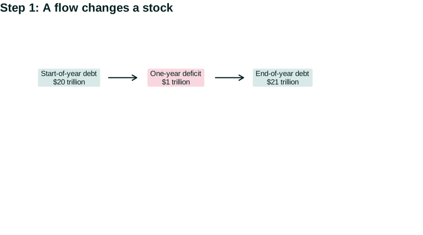
A budget deficit is a flow: over a stated period, government outlays exceed receipts under an accounting convention. Public debt is a stock of outstanding obligations at a point in time. A bathtub analogy helps only this far: the deficit is like net flow during a period; debt is like the level. Interest, asset sales, valuation, and the definition of debt add complications.

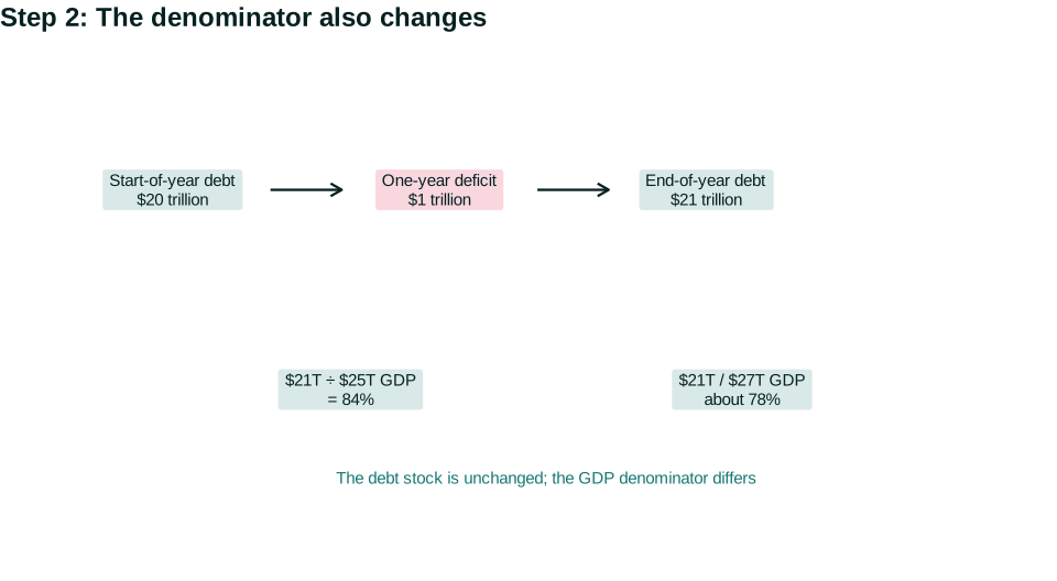
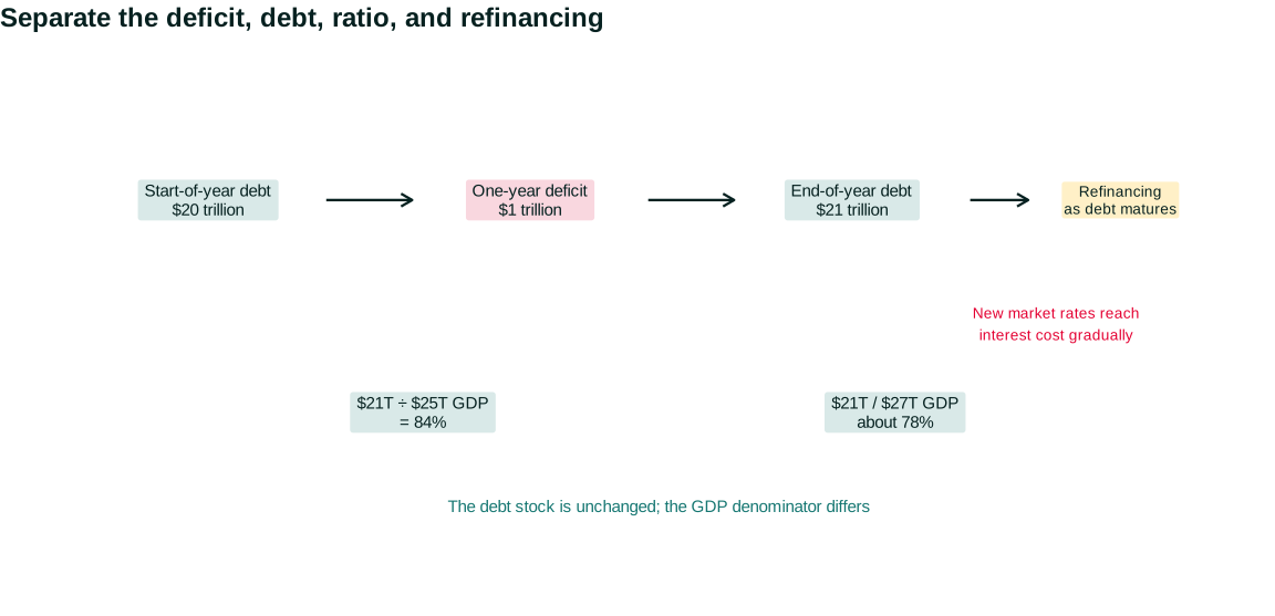
Suppose federal debt is $20 trillion at the beginning of a year and net borrowing is $1 trillion. Ignoring other changes, debt ends at $21 trillion. If nominal GDP is $25 trillion, the debt-to-GDP ratio is 84 percent. If GDP later grows to $27 trillion while debt remains $21 trillion, the ratio falls to about 78 percent without debt being repaid. Both numerator and denominator matter.

The debt-to-GDP ratio scales obligations by national income, but it is not a household debt-to-income ratio. The federal government is a continuing institution with taxing authority, a central bank, a currency, many creditors, and debt of different maturities. It does not need to retire all obligations at a biological endpoint. Nor does that mean it faces no constraint.

Interest cost depends on interest rates, maturity, inflation, and the debt stock. If much debt is fixed-rate and long-term, a market-rate increase affects interest expense gradually as securities mature and are replaced. If maturities are short, refinancing happens faster. Unexpected inflation can reduce the real value of fixed nominal debt but also raise future borrowing costs and redistribute from creditors.

Figure 9.6 keeps four objects separate. Step 1 turns a deficit flow during the year into a change in the debt stock. Step 2 introduces GDP as the denominator. The summary adds refinancing: a new market rate affects interest costs as existing securities mature, not as though the entire stock were a floating-rate credit card balance.

Step 1: Flow changes stock

An illustrative one-trillion-dollar deficit raises debt from twenty to twenty-one trillion dollars.

Step 2: Add the GDP denominator

The same debt stock equals different debt-to-GDP ratios when GDP differs.

Summary figure

Figure 9.6: A deficit, debt stock, debt-to-GDP ratio, and refinancing are related but distinct.

Open the live step-by-step figure

Use the figure as a sequence of questions. What period defines the deficit? Which debt concept is in the numerator? Which GDP measure and date define the denominator? How much debt matures soon? Only then ask what was financed and what risks follow. A large number without those definitions can provoke concern without supporting analysis.

Read a debt claim carefully

News reports often compare the federal debt with a very large dollar threshold. The number can be accurate and still uninformative without a denominator, definition, and maturity. “Gross federal debt” includes debt held by government accounts; “debt held by the public” answers a different question. Nominal dollars across decades are changed by inflation and economic growth. A serious comparison states which concept is used.

Consider a government with $24 trillion of debt held by the public. Assume the average effective interest rate on that debt is 3 percent, so annual interest is roughly $720 billion. If new market rates rise to 5 percent, interest expense does not instantly become $1.2 trillion because older fixed-rate securities remain outstanding. Each maturity and new borrowing is refinanced at then-current rates. The speed depends on the maturity structure.

Now suppose the government financed a project that raised future productive capacity and tax receipts. Its debt is higher, but so may be future GDP and fiscal capacity. Suppose instead that borrowing financed resources when the economy was already at capacity and mainly raised prices. The same initial accounting flow has different later consequences. Accounting cannot tell us the return on what was financed.

Creditors also differ. Households can hold Treasury securities directly or through pensions and mutual funds; banks use them as liquid assets; foreign institutions hold them for reserves and investment; the Federal Reserve holds securities as assets. Interest is an expense to the government and income to holders. Distribution depends on ownership and on how taxes adjust.

Currency denomination matters. A government owing debt in a currency it cannot issue faces exchange-rate and rollover risks different from the US federal government. But issuing one’s own currency does not create real resources. If the economy is at capacity, additional nominal spending can increase inflation or reallocate production. Monetary sovereignty changes financing risk; it does not abolish opportunity cost.

Political capacity matters too. A government may possess taxable resources yet fail to raise revenue because institutions cannot administer taxes or coalitions block action. A legal debt ceiling can create payment risk independently of long-run resource capacity. Calling such outcomes “market discipline” can obscure the political rule that generated them.

This is why fiscal space is conditional and institutional. Analysts should ask about expected growth, interest rates, maturity, currency, tax capacity, productive use, inflation, investor demand, political constraints, and the shock requiring response. A single debt threshold cannot incorporate all those dimensions.

Fiscal space is the capacity to use fiscal policy without creating unacceptable financing, inflation, institutional, or political risks. It is not one observed number. A country borrowing in its own currency with credible taxing capacity differs from a household, state government, or country owing foreign-currency debt. Productive capacity matters: financing can be available while real labor, energy, or materials are scarce.

Deficit debates often confuse three questions. Accounting asks how much the government borrowed. Causal analysis asks what the borrowing financed and what changed relative to no policy. Evaluation asks how benefits, taxes, inflation, interest payments, and risk are distributed across people and time. One answer cannot substitute for the others.

NoteMath Extension 9.6.1: A transparent debt-ratio change

If debt is initially 80 percent of GDP, nominal GDP grows 5 percent, and the government adds borrowing equal to 3 percent of initial GDP, the next ratio is approximately (83/105 = 79.0%). Growth in the denominator more than offsets the added debt in this example. Change growth to 1 percent and the ratio is (83/101 = 82.2%). This is arithmetic, not a sustainability verdict: interest, maturity, primary spending, taxes, inflation, and expectations remain to be analyzed.

Questions: Which changed condition accounts for the different ratios? Why does neither scenario prove that more borrowing is always safe or always harmful?

Federal borrowing capacity becomes especially important when state and local governments are required to retrench.

Questions

Question 9.6. Which statement is correct?

1. A deficit is a stock and debt a flow
2. Debt-to-GDP cannot fall if debt rises
3. A deficit is a flow and debt is a stock
4. Debt accounting settles policy desirability

Exercise

Flow and stock

Construct a numerical example in which debt rises but debt-to-GDP falls, then explain why it is not a sustainability verdict.

The model solution is available in the restricted instructor materials.

9.7 Austerity, the paradox of thrift, and US federalism

Austerity refers here to policy intended to reduce public deficits through spending cuts, tax increases, or both, especially during weak economic conditions. Whether a package is austere depends on timing and composition, not on one politician’s label.

For one household, cutting spending after income falls can preserve cash and reduce debt. For the economy as a whole, simultaneous cuts reduce sellers’ income. Chapter 6 called this the paradox of thrift. If government also cuts purchases and employment, aggregate income and tax revenue can fall further while benefit claims rise. The deficit may shrink by less than the initial cut suggests. This is not an identity that guarantees expansionary or contractionary effects; it is an aggregation mechanism whose strength depends on slack, trade, expectations, monetary policy, and confidence.

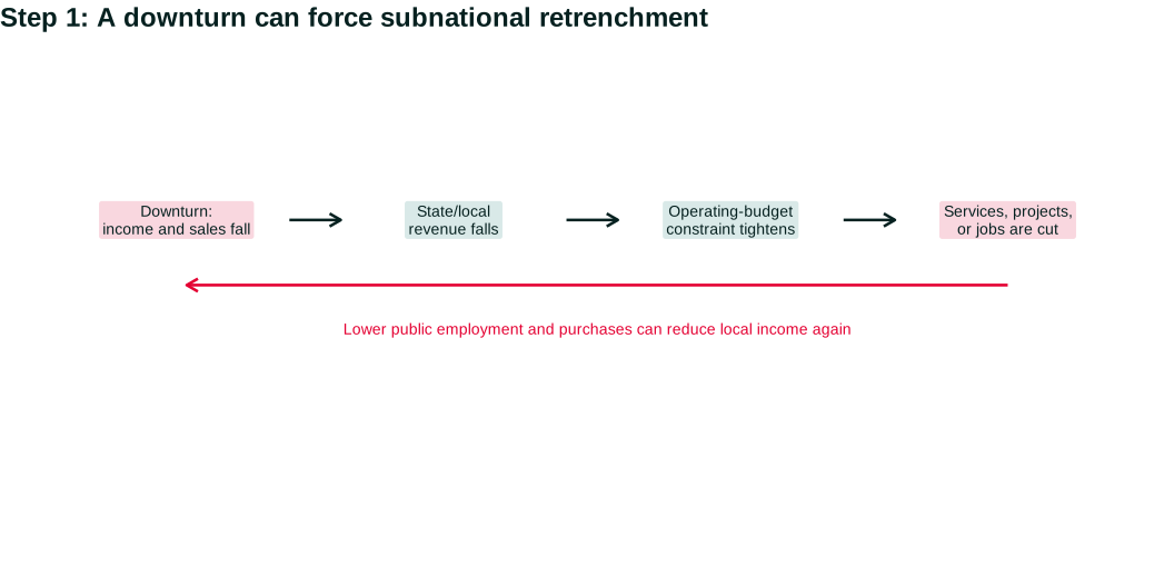
US federalism makes the mechanism concrete. The federal government, states, counties, cities, school districts, and public authorities divide responsibilities and revenue sources. State balanced-budget rules vary in detail, and states can use reserves or borrow for some capital purposes. Still, they face tighter operating constraints than the federal government. When income and sales-tax revenue fall, a state may cut services, delay projects, or reduce employment unless reserves and federal grants bridge the gap.

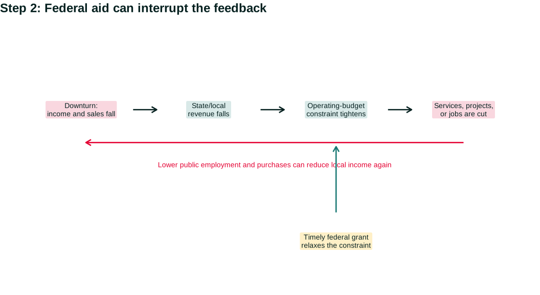
Figure 9.7 traces the adjustment. The first step shows the procyclical path: a downturn reduces revenues, operating-budget rules tighten the constraint, and service or employment cuts can reduce local income again. The second step adds federal grants as one possible interruption. The final step asks who bears risk under each route.

Step 1: The subnational feedback

A downturn can reduce state and local revenue, force cuts, and weaken local income further.

Step 2: Federal aid can interrupt the feedback

Timely federal grants can relax the state and local budget constraint.

Summary figure

Figure 9.7: US federalism assigns different adjustment powers and risks across levels of government.

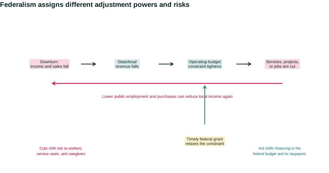
Open the live step-by-step figure

The arrow from federal aid is not a guarantee of stabilization. The amount, formula, allowable uses, advance or reimbursement structure, and expiration date determine whether aid reaches the binding constraint. State and local governments may also preserve reserves because future revenue is uncertain. Authority and expectations shape the adjustment alongside accounting.

Those cuts have distributional effects. Public-sector employment is an important source of work and mobility, including for women and Black workers. School, transit, health, disability, and housing cuts affect people who rely on public provision, not only the employees paid to provide it. A local cut can transfer risk to families doing unpaid care or traveling farther for services.

Federal aid can prevent subnational contraction, but design matters. Formula grants arrive differently from competitive grants. Maintenance-of-effort rules can preserve services but constrain state choices. Reimbursement can force cash-strapped governments to spend before receiving aid. Political representation affects which places gain voice. The Rules of the game principle is part of the causal mechanism.

Evidence from pandemic aid illustrates why purpose and counterfactual matter. One quasi-experimental study used differences in congressional representation to isolate variation in state and local aid. It estimated modest employment and aggregate-output effects in a period when state revenues and the broader economy proved more resilient than initially expected. That result does not show that grants never preserve services, improve health, or work differently in another downturn. It shows why the outcome, institutional setting, and alternative use of the funds must be specified. Pandemic state-and-local aid study

Return to the opening figure. The transfer spike shows federal capacity to support household resources; the employment drop shows that other public budgets did not automatically expand. Neither series alone measures total fiscal stance. A complete account adds purchases, taxes, transfers, state aid, loans, timing, and what would otherwise have happened.

The final step is to turn these distinctions into a repeatable evaluation rather than a yes-or-no judgment about “stimulus.”

Questions

Question 9.7. Why can state cuts amplify a downturn?

1. Public spending is someone else’s income
2. States issue the national currency
3. Federal grants never exist
4. Balanced-budget rules raise every service

Exercise

Federalism feedback

Trace how a state spending cut can change income, taxes, benefits, and federal aid during a downturn.

The model solution is available in the restricted instructor materials.

9.8 Evaluating a fiscal package

Begin with the problem. Is the economy facing deficient demand, a supply disruption, unemployment concentrated by place or industry, a public-health emergency, or a long-run capacity gap? Chapter 8 showed why the diagnosis matters. Demand support can raise employment after a spending collapse; after a negative supply shock, the same demand can intensify price pressure unless it also relaxes the constraint.

Then apply a common checklist:

Question	What to identify
Goal	Relief, stabilization, insurance, public provision, capacity, or distribution
Instrument	Purchase, public employment, transfer, tax change, grant, loan, or guarantee
Timing	Recognition, authorization, administration, spending, and production lags
Recipient and authority	Who qualifies, decides, implements, and can appeal
Demand mechanism	Direct purchase or induced private spending; likely leakages and offsets
Supply mechanism	Capacity created, scarce resources used, and bottlenecks
Distribution	Who receives services or income, pays taxes, earns interest, and bears inflation or cuts
Financing	Current taxes, borrowing, maturity, interest exposure, and institutional conditions
Evidence	Counterfactual, population, period, uncertainty, and external validity

No single row decides the package. A fast transfer can provide excellent relief yet have a modest multiplier. A public investment can yield large future benefits but arrive after a recession. A tax change can alter incentives and distribution even if short-run demand barely moves. A deficit can be appropriate in one state of the economy and risky in another.

Figure 9.8 turns the checklist into a sequence. First identify the problem, goal, and instrument. Then trace timing, authority, and the demand and supply mechanisms. Only after that should you judge distribution, financing, evidence, and limitations. Beginning with a favored instrument reverses the reasoning.

Step 1: Diagnose and choose

Fiscal evaluation begins with the problem, goal, and instrument.

Step 2: Trace implementation and mechanisms

The second stage identifies timing, authority, demand, and supply mechanisms.

Summary figure

Figure 9.8: A nine-question workflow for evaluating a fiscal package.

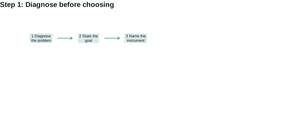
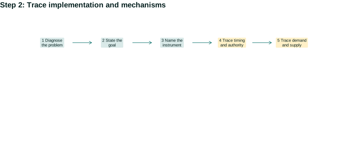
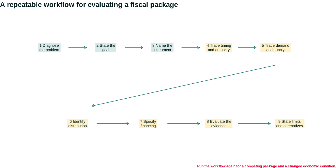
Open the live step-by-step figure

Apply the workflow twice: once to a demand-driven recession and once to a supply disruption. A rapid transfer may support spending in both. In the demand recession, firms with spare capacity can raise production. In the supply disruption, the same spending may raise prices unless the package also increases the constrained supply or protects essential consumption. The instrument has not changed; the mechanism and trade-offs have.

Then test a competing package. A public repair project may be too slow for immediate relief but valuable for resilience. A temporary tax reduction may reach payroll workers quickly but exclude people without earnings. Comparing alternatives makes opportunity cost visible and prevents the evaluation matrix from becoming a ceremonial checklist.

Finally, separate three kinds of conclusion. A descriptive conclusion reports what the statute authorized, who received payments, or how spending changed. A causal conclusion compares outcomes with a credible no-policy path. A normative conclusion judges the outcome using stated values—for example, stabilizing employment, protecting essential consumption, expanding public capacity, or limiting inflation and financing risk. Evidence can inform all three, but it cannot choose the values silently.

This separation also improves disagreement. Two analysts may agree about the accounting and causal estimate but value distribution or future risk differently. Or they may share a goal but disagree about implementation capacity and the counterfactual. Naming the exact point of disagreement is more useful than treating every fiscal debate as a contest between “more government” and “less government.”

Fiscal policy embodies the Principle of individual and societal interests. A household, firm, or state government may rationally cut spending to protect its own balance sheet. When many do so, aggregate income can fall and worsen their constraints. Collective fiscal institutions can interrupt that feedback, but their rules can exclude people, allocate power unevenly, or create future costs.

The chapter’s answer is conditional but usable. Fiscal institutions change demand directly through purchases and indirectly through taxes and transfers. They share risk through automatic rules and discretionary choices. Their effects depend on slack, recipient constraints, implementation, monetary conditions, and supply. Deficits are flows and debt is a stock; neither settles desirability. The next chapter examines a different authority: how the Federal Reserve’s interest-rate decisions reach financial conditions, spending, employment, and inflation.

Questions

Question 9.8. A good fiscal-package evaluation begins by…

1. assuming every shock is deficient demand
2. identifying the goal and disturbance
3. using one universal multiplier
4. ignoring distribution

Exercise

Evaluate a package

Apply the chapter checklist to a fiscal proposal and identify the most important missing evidence.

The model solution is available in the restricted instructor materials.

Seeing the principles in action

Principle	Example	Everyday Economics
Interdependence principle	Public purchases, taxes, transfers, and borrowing connect household, firm, government, and creditor budgets.	A government purchase becomes income for a worker or supplier.
Doing the best you can principle	Households and governments respond to shocks under liquidity, legal, administrative, and political constraints.	A city may cut services when revenue falls even as need rises.
Rules of the game principle — focal	Eligibility, tax schedules, procurement, federalism, and budget rules determine who can act and when.	Federal grants can relax a state’s balanced-budget pressure.
Trade-offs and opportunity costs principle	Relief, stabilization, public provision, and future capacity can compete for scarce resources and administrative attention.	A shovel-ready repair can arrive sooner than a new rail line.
Principle of gains from cooperation and conflict of interest	Risk sharing can preserve livelihoods while groups conflict over taxes, services, inflation, and interest payments.	A transfer protects a renter while financing choices affect taxpayers and creditors.
Principle of individual and societal interests — focal	Individually sensible spending cuts can collectively reduce income and worsen budget constraints.	Many households and governments saving at once can deepen a downturn.
Principle of aggregation and feedback — focal	One actor’s spending is another’s income, so fiscal changes can be amplified or offset.	A public wage supports purchases at nearby businesses.

Skills and learning objectives

• Classifying fiscal transactions
• Explaining automatic stabilizers
• Comparing context-dependent multipliers
• Distinguishing deficits from debt
• Evaluating federalism and distribution

Concepts to learn

• Fiscal policy
• Government purchases and transfers
• Automatic stabilizers
• Discretionary policy
• Fiscal multiplier
• Budget deficit and public debt
• Fiscal space
• Austerity and federalism

Glossary

Chapter 9 terms

fiscal policy

Government decisions and rules concerning purchases, public employment, taxes, transfers, and borrowing.

See also: government purchase; transfer payment.

government purchase

A government payment for a currently produced good or service that enters GDP directly.

See also: transfer payment.

transfer payment

A payment that changes the recipient’s resources without purchasing current production in that transaction.

See also: government purchase.

automatic stabilizer

A tax or spending rule that responds to economic conditions without new discretionary legislation.

See also: discretionary fiscal policy.

discretionary fiscal policy

A fiscal change requiring a new legislative or administrative decision.

See also: automatic stabilizer.

fiscal multiplier

The change in output relative to a policy-induced fiscal change under stated conditions and over a stated period.

See also: automatic stabilizer.

budget deficit

A flow during a period in which government outlays exceed receipts under a stated accounting convention.

See also: public debt.

public debt

A stock of outstanding government obligations measured at a point in time.

See also: budget deficit; debt-to-GDP ratio.

debt-to-GDP ratio

Public debt divided by annual GDP, used to scale a debt stock relative to national income.

See also: public debt.

fiscal space

Capacity to use fiscal policy without unacceptable financing, inflation, institutional, or political risks.

See also: public debt.

austerity

Policy intended to reduce public deficits through spending cuts, tax increases, or both, especially during weak conditions.

See also: budget deficit.

Flashcards

Why is a transfer not a government purchase?

It changes recipient resources without buying current production in that transaction; later recipient spending is behavioral.

What makes a stabilizer automatic?

Existing tax or benefit rules respond to economic conditions without a new discretionary law.

Deficit versus debt?

A deficit is a flow over a period; debt is a stock at a point in time.