GDP, Living Standards, and Fluctuations
Public working draft: This AI-assisted chapter draft is open for coauthor revision. Its Google Doc remains canonical during human drafting and review. Figures, quantitative claims, source rights, and teaching decisions still require human review.
Central question: How can one economy-wide total describe production, income, and spending—and what does it leave out?
By the end of this chapter, you should be able to: explain why value added prevents double counting; reconcile production, income, and final expenditure as three views of the same measured activity; classify expenditure without treating an accounting identity as a causal model; distinguish nominal from real and total from per-person GDP; read long-run growth and short-run fluctuations from the same data; and evaluate what GDP includes, excludes, and cannot tell us about living standards.
5.1 When production suddenly falls
In March 2020, the manager of a neighborhood restaurant faced a problem that had no good solution. Customers stopped entering the dining room. Public-health rules restricted how the business could operate. Some employees could not work because schools and care arrangements had closed; others worried about infection. The restaurant could try takeout, reduce hours, draw on cash, borrow, or close temporarily. Each option shifted risk among workers, owners, creditors, suppliers, customers, and families.
Similar decisions were taking place at factories, airlines, clinics, universities, construction sites, and millions of households. Some production stopped because demand disappeared. Some stopped because safe production was temporarily infeasible. Some work moved into homes and digital systems. Some care work moved out of paid institutions and into families. A single national total could not preserve every one of those stories. It could, however, tell us how much measured production changed.
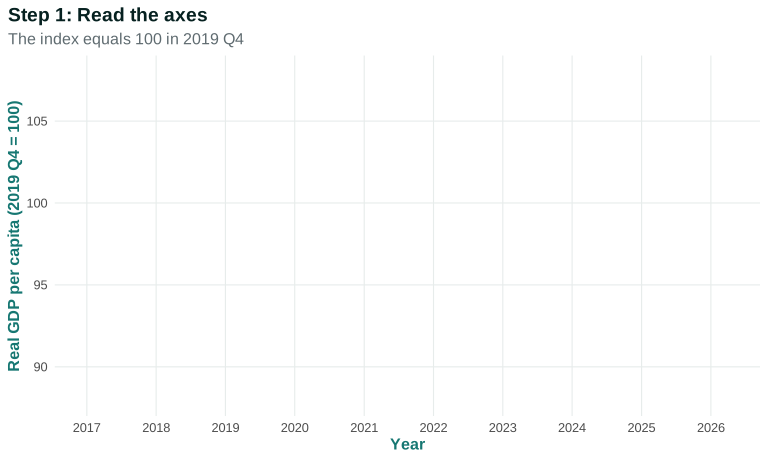
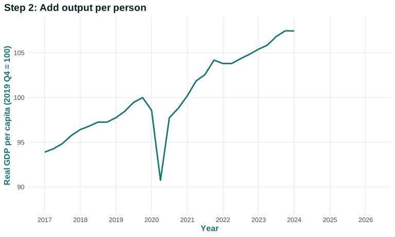
Figure 5.1 starts with real GDP per person, indexed so that the fourth quarter of 2019 equals 100. The horizontal axis records calendar time. The vertical axis does not show dollars. It shows production per person relative to the pre-recession quarter. A value of 95 would mean that measured real production per person was 5 percent below that baseline.
Open the live step-by-step figure
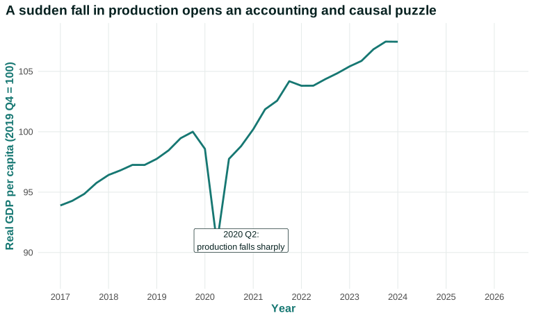
Compare three points. The index is 100 in 2019 Q4. It falls a little in 2020 Q1 and then to about 91 in 2020 Q2. It rises sharply in 2020 Q3, but a rising line does not mean that every worker, business, or community had recovered. It means that the measured national average was moving upward from a very low quarter. The level, the direction of change, and the distribution of recovery are three different questions.
The figure is descriptive. It shows the timing and size of the fall in one aggregate measure. It does not separate public-health constraints, voluntary avoidance of contact, income losses, government policy, disrupted supply chains, or differences among industries. Nor does it tell us whether an hour of unpaid care replaced an hour of paid care. A time series can locate a change without identifying its causes.
The National Bureau of Economic Research dates the most recent US recession from a monthly peak in February 2020 to a trough in April 2020. It uses a range of measures because a recession is a broad contraction in economic activity rather than a technical rule about GDP alone. The unusually deep and widely spread collapse was classified as a recession even though it was brief. Quarterly GDP and monthly recession dates therefore answer related but different questions.
This leaves us with our central question. How can one total compress the production of meals, health care, software, machinery, education, government services, and millions of other goods and services? Why can the same activity be recorded as production, income, and spending? And what disappears when we compress a diverse economy into one number?
The graph gives us a quantity to explain, but explanation must wait. Before we ask why total spending and production fell, we need the accounting rules that construct the total. We begin at the level of one product and one supply chain. TE 2.0 and UOE measurement sequence
Questions
Review the live step-by-step figure
Question 5.1. What does Figure 5.1 establish by itself?
- The pandemic caused every household’s income to fall equally
- Real GDP per capita fell sharply in 2020 Q2
- Consumer spending was the only cause
- Production never recovered
Exercise
Describe before explaining
Use Figure 5.1 to state one claim about the level and one about the timing of the 2020 contraction; then name two mechanisms the figure cannot distinguish.
The model solution is available in the restricted instructor materials.
5.2 Production and value added
What belongs in domestic production?
Gross domestic product is the market value of final goods and services produced within a country during a stated period. Every part of that definition does work.
Gross means that the wearing out of buildings, machines, software, and other capital has not yet been subtracted. Domestic assigns production to the country where it occurs, not to the nationality of the worker or owner. Production refers to goods and services newly produced during the period, not the resale of an existing house or share of stock. Final distinguishes output purchased for final use from inputs that will be used to produce something else. During a period reminds us that GDP is a flow—production per quarter or per year—not a stock of accumulated wealth.
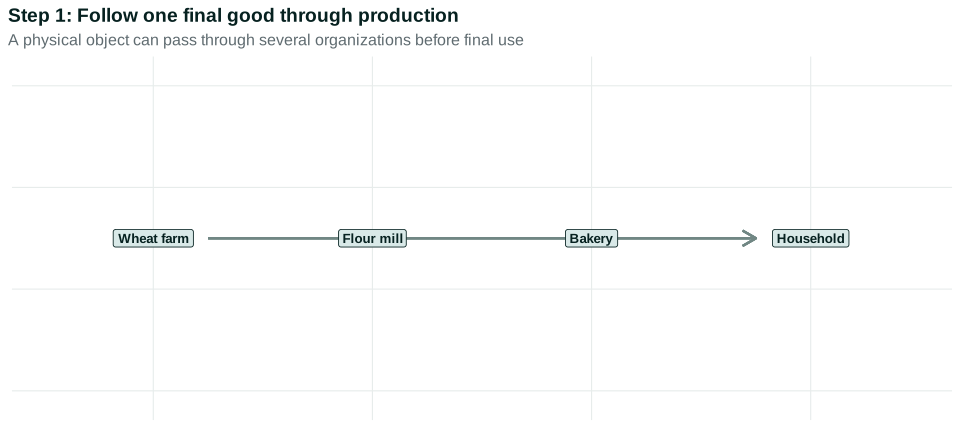
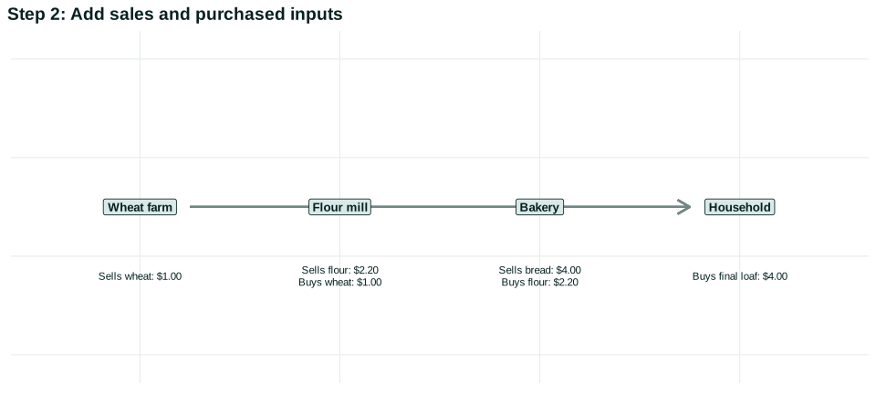
Suppose a wheat farmer sells grain to a mill, the mill sells flour to a bakery, and the bakery sells bread to a household. If we add every sale, we count the wheat inside the flour and then count both again inside the bread. GDP avoids this duplication by counting final output or, equivalently, by adding the new value created at each stage.
| Producer | Sales | Purchased intermediate inputs | Value added |
|---|---|---|---|
| Wheat farm | $1.00 | $0.00 | $1.00 |
| Flour mill | $2.20 | $1.00 | $1.20 |
| Bakery | $4.00 | $2.20 | $1.80 |
| Total | $7.20 | $3.20 | $4.00 |
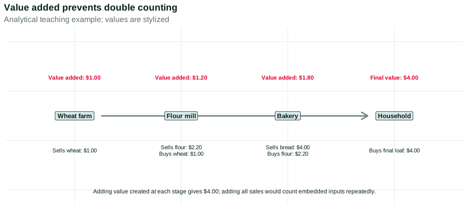
Value added is a producer’s sales minus the cost of intermediate goods and services purchased from other producers. The farm adds $1.00, the mill $1.20, and the bakery $1.80. Their value added sums to $4.00, exactly the price of the final loaf. The $7.20 sum of sales is not wrong as a record of transactions; it is wrong as a measure of newly produced final value because it counts embedded inputs repeatedly.
Figure 5.2 teaches the same arithmetic as a chain. Each box shows the producer’s contribution, not the producer’s total revenue. The step sequence matters because students often see the final $4 loaf and overlook the multiple organizations and workers that made it possible.
Final and intermediate describe uses, not physical objects
A good is not permanently final or intermediate. Flour bought by a bakery is an intermediate input. Flour bought by a household for home cooking is a final consumption good. A pickup truck purchased by a delivery company is business investment; the same model purchased by a household for personal use is consumption. What matters is the use in the accounting period.
Inventory is especially important. If a bakery produces a loaf in December but sells it in January, the December production does not vanish. The unsold loaf enters inventory investment in December. When it is sold in January, the fall in inventory offsets the consumption sale so the same production is not counted twice. This treatment makes the production and expenditure accounts agree across time, although statisticians must estimate inventories with imperfect information.
Used goods illustrate the boundary in another way. The resale price of a used car is not current production, because the car was counted when it was first produced. A dealer’s current service—inspection, marketing, financing assistance, or warranty provision—can add current value. Likewise, buying shares transfers ownership of a financial asset; the brokerage service is production, but the share price is not GDP.
Value added becomes income, but not necessarily equal income
Value added is divided among claims. A business may pay wages and salaries, payroll taxes, rent, interest, production taxes, and profits. Owners decide how much profit to distribute and how much to retain. Workers can create value without receiving an equal amount in wages. The accounting does not settle whether the division is fair or efficient.
The Chapter 3–4 model makes this point visible. Output per worker can be divided between the real wage and profit per worker. GDP aggregates the value created across firms and institutions, while the income account records who receives claims on that value. Market power, bargaining institutions, ownership, discrimination, and public rules affect the division even when the accounting total is unchanged.
The production boundary also depends on institutions. Government-provided schooling, fire protection, or public health services may not have a market sale price. National accountants generally value much government production by the cost of the labor, buildings, and other inputs used. This makes public services visible in GDP, but it does not directly measure their quality or social value. A highly effective and an ineffective program with the same measured cost can contribute the same amount to GDP.
Classification becomes harder when organizations bundle products. A free phone app may be supported by advertising, data collection, or a paid service sold to another business. A hospital bill can combine professional labor, medication, equipment, insurance negotiation, and administrative services. A university produces teaching, research, credentials, and community services that cannot be observed as identical physical units. Statisticians must choose observable prices and quantities while avoiding the pretense that every service is homogeneous.
Global production creates another boundary problem. A US-designed product can contain imported components, domestic logistics, foreign software work, and profits paid to owners in several countries. Domestic GDP counts value added within US borders. Gross national income instead follows income accruing to residents. Neither measure alone maps the entire supply chain or tells us where authority and environmental burden sit. The word “domestic” should therefore trigger a location question, not a nationality story.
Finally, informal and illegal market activity presents measurement challenges. A transaction can be economically productive under the conceptual boundary yet missing from surveys and tax records. Conversely, a recorded cash transfer may not correspond to new production. Estimates use multiple sources, imputations, and reconciliation. The boundary is conceptually defined, but observation is imperfect.
We can now construct total production without double counting. The next step is more surprising: the same $4 loaf can be viewed not only as final production, but also as final spending and as income generated along the chain.
Questions
Question 5.2. Why use value added?
- To count every transaction twice
- To count each producer’s new contribution
- To measure household happiness
- To exclude wages
Exercise
Value added
For a $2 input sold to a producer who sells a $7 final good, calculate value added at each stage and explain why adding both sales overstates GDP.
The model solution is available in the restricted instructor materials.
5.3 Three views of the same production
One transaction, three records
When a household buys the $4 loaf, three events are recorded. A final good worth $4 has been produced. The household has spent $4. The production process has generated $4 of value added that becomes income claims. These are not three separate additions to GDP. They are three views of the same completed economic activity.
| View | Question | Amount in the bread example |
|---|---|---|
| Production | How much final value was produced domestically? | $4.00 |
| Expenditure | Who purchased the final output? | $4.00 |
| Income | What labor, ownership, tax, and other income claims were generated? | $4.00 |
In a real statistical system, the estimates do not line up perfectly at first. Production surveys, household and business expenditure data, tax records, and income reports arrive at different times and contain measurement error. Statistical agencies revise estimates and report a discrepancy rather than pretending every source agrees immediately. The identity describes the completed accounts after definitions and reconciliation; it does not imply perfect raw data.
Classifying final expenditure
The expenditure view is often written
\[Y = C + I + G + X - M.\]
Here \(Y\) is measured domestic output. \(C\) is household consumption. \(I\) is investment in newly produced capital, residential structures, and inventories. \(G\) is government consumption and investment—purchases of currently produced goods and services. \(X\) is exports, which are domestically produced and purchased from abroad. \(M\) is imports.
This national income identity is a classification rule. To use it correctly, ask two questions in order: Was the item newly produced during the period? If so, was it produced domestically? The category of the purchaser comes next.
Consider a small economy with the following final expenditures during a week:
| Transaction | Initial category | Domestic-production adjustment | Contribution to domestic GDP |
|---|---|---|---|
| Households buy domestic meals | C = $500 | none | $500 |
| A firm buys a domestically made oven | I = $300 | none | $300 |
| A city buys domestic repair services | G = $200 | none | $200 |
| Foreign customers buy domestic software | X = $150 | none | $150 |
| Households buy imported phones | C = $250 | M = −$250 | $0 |
| Total domestic production | $1,150 |
Imports are subtracted because they may already appear in consumption, investment, or government purchases. The subtraction does not say that imports are harmful, that the buyer made a mistake, or that the imported good has negative value. It removes foreign production from a domestic production total. Domestic retailing, warehousing, and transportation services associated with the imported phone remain domestic value added.
Everyday Economics 5.1
Buying an imported laptop raises measured consumption, but its imported value is subtracted in \(M\). Domestic retail and delivery services remain in US GDP.
Purchases are not the same as transfers
Government purchases pay for current goods and services: a teacher’s work, a bridge repair, a vaccine, or a computer for a public office. A Social Security payment, unemployment benefit, or scholarship payment is a transfer of purchasing power. The transfer is not counted directly in \(G\) because it is not payment for current production. When the recipient later buys a final good, that purchase enters the relevant expenditure category.
This distinction prevents a common error. Saying that a transfer is not in \(G\) does not say it is economically unimportant. Transfers can alter disposable income, consumption, poverty, risk, and bargaining positions. They become part of the causal story in Chapter 6. Chapter 5’s accounting question is narrower: where does the completed transaction appear?
The same care is needed with investment. In everyday speech, buying a stock or a bond is an investment. In the national accounts, it is mainly an exchange of financial claims. Macroeconomic investment refers to newly produced capital, residential construction, and inventory accumulation. A new factory machine contributes to current production; the purchase of an existing corporate share does not produce a new machine.
Identity is not explanation
Because \(Y\) and \(C+I+G+X-M\) are two records of the same realized activity, they must be equal. But the equality does not tell us what would happen if government purchases rose, households cut consumption, or firms changed investment plans. It does not tell us which actor adjusts, how quickly production responds, whether prices change, or what monetary and fiscal institutions do.
For example, if \(G\) rises by $100, it is incorrect to infer from the identity alone that \(Y\) must rise by $100. Taxes might change, imports might rise, households might alter spending, the central bank might respond, or the economy might be at capacity so that prices rise. Conversely, a fall in consumption may coincide with an unintended rise in inventories before firms reduce production. Accounting organizes what happened. A model and evidence are needed to explain adjustment and causation.
The three-view equality is nevertheless powerful. It tells us that one person’s expenditure is revenue somewhere, and revenue ultimately supports income claims. It lets statisticians check inconsistent sources. It also disciplines political arguments: components cannot be added or subtracted casually without asking where the offset appears.
The income view keeps workers, owners, and government visible
The income account is sometimes compressed into the phrase “income generated by production.” For analysis, it helps to unpack the recipients. Employee compensation includes wages, salaries, and employer contributions to benefit programs. Proprietors receive income from unincorporated businesses. Owners of corporations may receive distributed profits or retain earnings inside the firm. Governments receive taxes on production and imports, net of relevant subsidies. Depreciation records the estimated use of capital that makes gross output larger than net output.
These categories connect accounting with the class structure developed in Chapter 4. A worker’s wage is a claim generated by production, but ownership gives access to profit and asset claims. A small-business owner may combine labor income and ownership income in one person. A pension fund may hold corporate shares on behalf of workers, while control rights remain concentrated in financial institutions and corporate governance. National accounts classify flows; they do not fully describe authority.
The distinction matters for interpreting recovery. If GDP returns to its previous level while employee compensation, proprietors’ income, and corporate profits follow different paths, “the economy recovered” conceals who received the restored income. Distributional accounts, household surveys, tax data, and balance sheets are needed alongside GDP. The production total is a starting point for that investigation, not a substitute for it.
The circular flow is therefore more than a picture of money traveling in a loop. Households supply labor and own assets; firms organize production and make employment and investment decisions; governments tax, transfer, purchase, regulate, and produce; financial institutions create contracts that move claims across time; and the foreign sector buys exports and supplies imports and finance. The GDP identity selects current production flows from this larger institutional system.
We have built the total. We next ask how to compare it across time, when both quantities and prices change, and across populations of different size.
Questions
Question 5.3. Which is a correct interpretation of Y=C+I+G+X-M?
- It is an accounting classification of measured output
- Every dollar of G always raises Y by one dollar
- Imports reduce welfare
- Consumption creates no income
Exercise
Classify expenditure
Classify four transactions as C, I, G, X, M, or excluded, and explain why imports are subtracted rather than treated as bad production.
The model solution is available in the restricted instructor materials.
5.4 Nominal, real, total, and per person
Why current-dollar growth can mislead
Nominal GDP values current production at current prices. It is the dollar amount that appears in current contracts, tax bases, revenues, and debt ratios. But nominal GDP can rise when more is produced, when prices rise, or both.
Imagine an economy that produces only meals and bicycles.
| Good | Year 1 quantity | Year 1 price | Year 2 quantity | Year 2 price |
|---|---|---|---|---|
| Meals | 100 | $10 | 105 | $11 |
| Bicycles | 10 | $200 | 11 | $210 |
Year 1 nominal GDP is $1,000 of meals plus $2,000 of bicycles, or $3,000. Year 2 nominal GDP is $1,155 plus $2,310, or $3,465. Nominal GDP has risen 15.5 percent. Yet quantities rose by only 5 percent for meals and 10 percent for bicycles. Part of the nominal increase reflects higher prices.
Real GDP uses a price-index procedure intended to remove the effect of the overall price change and track quantities. A simple classroom calculation can value both years at Year 1 prices. Year 2 production would then be $1,050 of meals plus $2,200 of bicycles, or $3,250. Measured at those fixed prices, quantity growth is about 8.3 percent rather than 15.5 percent.
Actual US accounts use chain-type quantity indexes rather than keeping one distant base year’s prices forever. Relative prices change: computers become cheaper relative to many services, new goods appear, and consumption patterns shift. Chain methods update weights over adjacent periods. The essential intuition is the same: a real measure tries to compare quantities while preventing an overall rise in prices from masquerading as more production.
Math Extension 5.4: A simple GDP price index
In the two-good example, the ratio of Year 2 nominal GDP to Year 2 output valued at Year 1 prices is $3,465/$3,250 = 1.066. Multiplying by 100 gives a simple price index of about 106.6. This fixed-base calculation is useful for arithmetic, but official chain-type measures handle changing expenditure weights more carefully and are not generally additive in the same way as current-dollar components.
Questions: If bicycle prices fell while meal prices rose, why would the choice of fixed weights matter more? What information does the price index discard when it compresses two price changes into one number?Total output and output per person
Suppose real GDP grows by 3 percent while population grows by 2 percent. Total real production has risen substantially, but real GDP per person rises by only about 1 percent. Dividing by population helps compare average material resources across time or countries of different size.
Per-person GDP is still an average. If production and income gains accrue mainly to owners of wealth or highly paid workers, GDP per person can rise while the median person’s income changes little. If working hours rise sharply, more output per person may come with less leisure. If environmental damage grows, current production can rise while future productive capacity or health deteriorates.
Four labels therefore answer four questions:
| Measure | Best suited to asking | Does not answer by itself |
|---|---|---|
| Nominal GDP | What is the current-dollar value of production and income? | How much more was physically produced? |
| Real GDP | How did aggregate quantities change? | How did output change per resident? |
| Nominal GDP per person | What is current-dollar production per resident? | How much of the change is prices? |
| Real GDP per person | How did average quantity-based production per resident change? | Who received the gains or whether well-being rose? |
The appropriate denominator can also differ. GDP per resident is useful for living-standard comparisons. GDP per worker or per hour is useful for productivity. Total GDP may matter for the tax base, emissions, public capacity, or geopolitical influence. No denominator is universally correct; the question determines the measure.
Current-dollar measures remain necessary even when we care about quantities. A borrower promises nominal dollars, not “real GDP units.” Tax brackets, business revenue, wages, and government budgets are initially recorded in current dollars. Inflation adjustment answers whether purchasing power or production quantity changed; it does not erase the nominal contracts through which gains and losses are distributed.
Nor does “real” mean “true” while nominal means “false.” Real GDP is a constructed quantity index based on observed expenditures, prices, classification rules, and methods for products whose quality changes. It is better suited to a quantity question because of that construction. Nominal GDP is better suited to some financing and current-budget questions. Good measurement begins by naming the question rather than ranking one statistic universally above another.
This section has separated price change, quantity change, and population change. We can now read long-run growth and short-run contractions in the same real series without confusing them.
Questions
Question 5.4. Real GDP differs from nominal GDP because it…
- removes population growth
- adjusts for changes in the overall price level
- measures median income
- excludes government
Exercise
Four GDP measures
Given nominal GDP, a price index, and population in two years, calculate nominal growth, real growth, and real per-person growth.
The model solution is available in the restricted instructor materials.
5.5 Growth and business-cycle fluctuations
The same series contains different time horizons
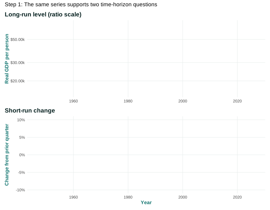
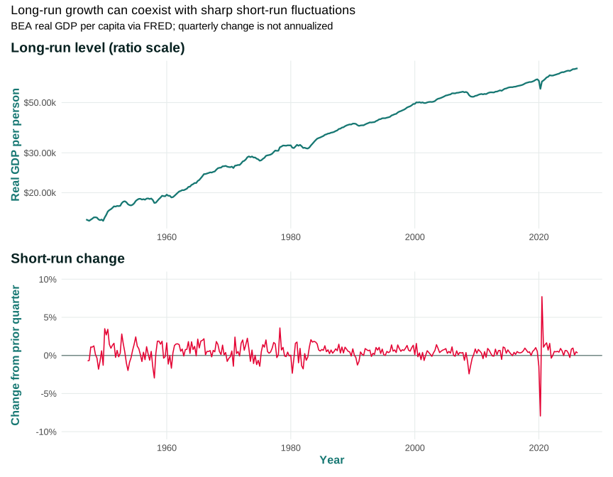
US real GDP per person has risen greatly over the long run, but the path is not smooth. Figure 5.3 uses the same pinned BEA series in two panels. The upper panel displays the level on a ratio scale: equal vertical distances represent equal proportional changes. The lower panel displays the percentage change from one quarter to the next. A long-run level and a short-run growth rate are not interchangeable.
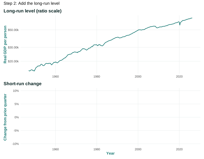
Open the live step-by-step figure
In the upper panel, the long-run rise dominates. In the lower panel, the line repeatedly crosses zero. A negative quarterly change is a contraction from the previous quarter. A positive change is expansion from the previous quarter. Positive growth after a deep fall does not guarantee that the level has returned to its previous path.
A business cycle is the irregular sequence of expansions and contractions in aggregate economic activity around its longer-run path. “Cycle” is a potentially misleading word because the movements do not arrive on a fixed timetable or with a fixed size. Wars, financial crises, public-health events, technology, policy, energy prices, expectations, and interactions among sectors can produce very different episodes.
The NBER identifies peaks and troughs retrospectively using production, income, employment, and spending evidence. It does not mechanically declare a recession whenever real GDP falls for two quarters. A two-quarter shortcut may sometimes match the historical dating, but it is not the US dating procedure. The delay is a feature of measurement under uncertainty: early data are incomplete and revised. NBER business-cycle dating
Seasonal adjustment, annualized rates, and revisions
Macroeconomic headlines often compare growth rates that use different conventions. A quarter-to-quarter rate compares one quarter with the immediately preceding quarter. An annualized quarterly rate asks how much output would change over a full year if that one-quarter pace continued for four quarters. Annualizing makes quarterly growth rates comparable with familiar annual rates, but it can make an unusual quarter look spectacularly large. The lower panel of Figure 5.3 deliberately uses the simpler nonannualized change from the previous quarter.
Seasonal adjustment answers another question. Retail sales normally rise before holidays, construction changes with weather, and schooling follows calendars. A seasonally adjusted series estimates what remains after recurring seasonal patterns are removed. It does not remove recessions, one-time shocks, or every calendar effect. Comparing an adjusted quarter with an unadjusted quarter can therefore create an apparent difference that is purely definitional.
Early GDP estimates use incomplete information. The BEA releases successive estimates as more surveys, tax records, and administrative data arrive. It later incorporates annual and comprehensive updates that can revise historical levels and growth. Revision is not evidence that the agency casually changes the answer. It is part of estimating a large, changing economy from multiple sources. Responsible analysis records the data vintage, especially when a claim depends on what policymakers knew at the time. BEA NIPA Handbook
This creates a useful evidence-reading routine. Before interpreting a growth number, ask: Is it nominal or real? Total or per person? A level or a rate? If a rate, annualized or not? Seasonally adjusted? Which vintage? Those questions prevent many disagreements that are really comparisons of unlike measures.
Production losses are distributed unequally
An aggregate decline can combine stable salaries for some workers, layoffs for others, profit losses for some businesses, increased profits for others, and increased unpaid work inside households. People with liquid savings, stable benefits, home equity, family resources, union protection, or access to credit have more ways to absorb an interruption. Renters with little cash, workers with irregular schedules, undocumented workers, and owners of small businesses tied to one place may face narrower options.
Class therefore affects both exposure and recovery. Ownership provides a claim on profits and assets, but owners also differ dramatically in scale and access to finance. Wage dependence makes job loss especially risky when health insurance or legal status is connected to employment. Race, gender, disability, citizenship, and place intersect with these positions through occupational sorting, discrimination, care responsibilities, transportation, housing, and unequal public services.
GDP tells us the size of the aggregate production change. It does not automatically tell us the counterfactual—what production would have been without the shock—or the persistence of losses. Interrupted schooling, long unemployment, business closure, delayed investment, and health damage can influence later capacity. Conversely, new technology or public investment can raise future production. Distinguishing a temporary movement from a change in the longer-run path requires more evidence and a model.
The same series therefore supports two lessons. Long-run growth can transform material possibilities. Short-run fluctuations can impose large and unequal costs even when the long-run line later rises. Neither lesson makes GDP a complete measure of living standards.
Questions
Question 5.5. A business-cycle contraction is…
- the same as lower long-run capacity
- a broad decline in aggregate activity
- always shared equally
- defined only by stock prices
Exercise
Trend and cycle
Sketch a rising trend with a temporary recession and explain why a return to growth need not restore every person’s lost income.
The model solution is available in the restricted instructor materials.
5.6 What GDP leaves out
A production boundary is not a welfare boundary
GDP is often criticized for failing to measure happiness, fairness, freedom, or sustainability. That criticism is useful only if we are precise. GDP was not designed as a complete measure of those outcomes. It measures production inside a defined boundary. The important question is how the boundary affects comparisons and decisions.
Consider care work. Paying a childcare center generally adds measured market production. A parent or relative providing similar care without pay is generally outside the central GDP measure. If a family shifts from paid care to unpaid care, measured GDP can fall even if the child receives the same number of care hours. The economic burden has moved into the household, not disappeared.
The American Time Use Survey documents time spent on household activities and care that market accounts do not directly price. These activities are essential to the reproduction of daily life and the paid workforce. Their distribution is shaped by gender, household income, work schedules, disability, family structure, migration, and public provision. Treating them as outside GDP is an accounting convention, not a claim that they have no value. BLS American Time Use Survey
| Activity or outcome | Typical GDP treatment | What remains unresolved |
|---|---|---|
| Paid childcare service | Included as current production | Quality, affordability, worker pay, and access |
| Unpaid family childcare | Usually outside the central production boundary | Time cost, well-being, and distribution within households |
| Leisure | Not added as production | Whether more output required longer or more intense work |
| Pollution cleanup | Cleanup services may raise GDP | The original environmental and health loss |
| Resource depletion | Extraction contributes to current GDP | Loss of natural assets and future options |
| Government service | Often valued by input cost | Quality, reach, rights, and outcomes |
| New digital service at zero price | Some production costs may be counted | Consumer benefit, data extraction, privacy, and quality |
Environment, depletion, and defensive expenditure
If a factory produces more output while imposing pollution costs that are not priced, GDP records the market production but does not subtract the full external damage. If a hurricane destroys homes, the loss of existing wealth is not the same as a fall in current GDP. Rebuilding later can raise measured production. It would be wrong to conclude that destruction improved well-being because rebuilding expenditure increased.
Environmental and national-accounting researchers construct satellite accounts and asset measures to supplement GDP. They can track energy use, emissions, ecosystems, minerals, forests, or environmental services without pretending that every loss has one uncontroversial dollar value. The accounting challenge is not a reason to ignore biophysical constraints. It is a reason to present production, asset depletion, emissions, health, and distribution as distinct measures.
Quality, public services, and institutional access
Measuring services is difficult because quantity and quality are intertwined. A medical visit, college course, legal service, or software subscription is not a standardized physical unit. If the price rises because quality improves, treating the full rise as inflation understates real output. If price rises without quality improvement, treating it as more output overstates progress. Statistical agencies use methods and assumptions that should be documented and revised.
Government services create a related problem. A public defender, election office, or disability-benefit administrator contributes to institutional access, but input costs do not tell us whether people receive equal treatment, timely service, or meaningful voice. Chapter 1 introduced capabilities and political participation precisely because production resources and the ability to use them are different outcomes.
Distribution and security
GDP per person can rise while economic insecurity rises. Two societies with the same average production can differ in unemployment risk, wage dispersion, wealth, housing, health coverage, exposure to debt, discrimination, union representation, and public insurance. The Lorenz curve in Chapter 4 showed why an average cannot reveal the distribution of wages and profits. GDP adds the production total but does not remove that limitation.
The Principle of individual and societal interests helps us avoid two opposite errors. Market prices do not automatically equal social value, because prices can omit external effects, unequal rights, and unpaid work. But an analyst should not replace GDP with an undefined personal judgment called “well-being.” A serious dashboard states each measure’s concept, unit, source, population, and limitation.
The right conclusion is not “GDP is bad.” It is: use GDP for the question it answers, and place it beside measures needed for the questions it does not answer. That measurement discipline prepares us to distinguish production, welfare, distribution, sustainability, and capability rather than asking one number to do every job.
Data Extension 5.6.1: Time use and the production boundary
The Bureau of Labor Statistics’ American Time Use Survey asks people to report how they spent a diary day. Its categories include paid work, household activities, care for household and nonhousehold members, education, purchasing, and leisure. In 2025, the published summary reported that 81 percent of people engaged in household activities on an average day and spent about two hours on them. Participation and time differed by gender, age, employment, and whether children were present.
These numbers do not provide a ready-made dollar addition to GDP. A minute of care has no unique market price, respondents may classify activities differently, and simultaneous activities are difficult to value. Applying the wage of a professional caregiver to every unpaid care hour would answer one replacement-cost question; applying the caregiver’s forgone wage would answer an opportunity-cost question. The two methods need not agree.
The survey nevertheless makes an otherwise hidden input visible: time. Imagine that a household replaces ten weekly hours of purchased childcare with ten hours provided by a parent. Market expenditure and measured GDP may fall. The child’s care hours may remain constant, but the parent’s leisure, paid work, sleep, or other household production must adjust. The distribution within the household can change even when the family makes the best choice available under its income, schedule, and care constraints.
To investigate the boundary responsibly, compare groups without treating gender, class, race, or family structure as competing explanations. Paid-leave rules, school schedules, childcare prices, disability services, wages, immigration status, and household wealth shape who performs unpaid work and what alternatives are feasible. An observed time-use gap describes allocation under these institutions; it does not by itself reveal preference or identify a single cause.
Use the BLS American Time Use Survey tables to choose two household-activity or care measures. Record the population, year, unit, and whether the statistic is for all people or only participants. Then answer:
- What production or capability does the activity support?
- How would GDP change if an unpaid hour became a paid market service, holding the underlying service constant?
- What additional evidence would you need to evaluate the change in well-being and bargaining power?
Questions
Question 5.6. Which can raise GDP without proving well-being rose?
- Rebuilding after a destructive storm
- More leisure with unchanged production
- Unpaid care replacing paid care
- Cleaner air with no market transaction
Exercise
GDP boundary audit
Compare a paid care service, unpaid family care, pollution cleanup, and leisure. State how GDP treats each and what additional measure you would want.
The model solution is available in the restricted instructor materials.
5.7 From accounting to explanation
We can now reconcile the chapter’s central pieces. Value added prevents double counting. Production, income, and final expenditure are three accounting views of the same measured activity. Nominal, real, total, and per-person measures answer different comparison questions. Growth and recession describe changes in aggregate activity, while GDP’s boundary leaves important dimensions of living standards to other measures.
The Rules of the game principle applies directly. National-accounting standards determine boundaries, classifications, seasonal adjustments, revisions, and the treatment of government and nonmarket production. Those rules make comparison possible. They also create obligations for transparency: users should be able to learn what was counted and how estimates changed.
The Principle of aggregation and feedback creates the bridge to Chapter 6. The GDP identity records realized transactions. It does not tell us how plans become outcomes.
| Type of statement | Chapter 5 example | What must be added for explanation? |
|---|---|---|
| Accounting identity | Realized output equals realized income and final expenditure | Nothing makes the equality causal |
| Behavioral relationship | A household may spend part of added disposable income | Evidence about choices and constraints |
| Causal claim | A spending change caused production to change | A mechanism, counterfactual, and identification strategy |
| Aggregation feedback | Lower spending reduces income and can induce further lower spending | Timing, leakages, institutional responses, prices, and capacity |
One household can reduce spending and accumulate cash. But if many households reduce spending together, businesses lose revenue. They may cut hours, orders, or investment. Those changes reduce other people’s income, which can generate further spending reductions. The completed accounts will still show expenditure equal to income. The explanation lies in the sequence of decisions connecting one round to the next.
Chapter 6 therefore adds behavior without changing the accounting. It asks: How can one person’s decision to spend less reduce other people’s income?
Before moving on, apply a four-part audit to any GDP claim. First, identify the accounting concept: production, income, expenditure, or a component. Second, identify the transformation: nominal or real, total or per person, level or growth rate. Third, identify the evidentiary claim: description, comparison, or causation. Fourth, identify what distributional or institutional information the aggregate omits. A sentence that survives all four questions is much less likely to ask GDP to prove something it cannot.
For example, “real GDP per person fell sharply in 2020 Q2” is a descriptive claim supported by Figure 5.1. “The fall reduced every household’s material well-being by the same percentage” fails the distribution test. “Government restrictions caused the entire decline” fails the causal-evidence test. “The subsequent positive growth rate immediately restored the pre-pandemic path” confuses a rate with a level. The discipline of measurement is itself a transferable economic skill.
This audit also clarifies why revisions to GDP do not automatically overturn every conclusion. A small revision may leave the direction and broad timing of a contraction intact while changing its reported magnitude. A large revision may change comparisons across episodes. Analysts should distinguish conclusions robust to plausible revisions from claims that depend on a particular early estimate. That habit will matter when we evaluate inflation, employment, fiscal policy, and growth later in the book.
Seeing the principles in action
| Principle | Example | Everyday Economics |
|---|---|---|
| Interdependence principle | Production links workers, firms, households, government, and trading partners through value added and expenditure. | Your purchase becomes revenue and income elsewhere. |
| Doing the best you can principle | Households and firms make plans using the information and resources they have, while GDP records completed production. | A business may cut inventories when expected sales fall. |
| Rules of the game principle — focal | National-accounting standards determine boundaries, classifications, and revisions. | Unpaid care and a purchased care service can be treated differently in GDP. |
| Trade-offs and opportunity costs principle | Production uses labor, capital, time, and natural resources that cannot simultaneously serve every alternative. | Rebuilding after a storm diverts resources from other projects. |
| Principle of gains from cooperation and conflict of interest | Specialized production creates gains while wages and profits divide value added. | A supply chain raises output but participants may disagree over its proceeds. |
| Principle of individual and societal interests — focal | Market value is not identical to social value; unpaid care and environmental damage expose the difference. | A paid replacement raises GDP even when the underlying need is unchanged. |
| Principle of aggregation and feedback — focal | GDP aggregates millions of transactions, but explanation requires feedback among spending, income, and production. | One household’s spending is another actor’s income. |
Skills and learning objectives
- Reading an indexed empirical graph
- Calculating value added without double counting
- Distinguishing an accounting identity from a causal relationship
- Comparing nominal real total and per-person measures
- Evaluating GDP as a bounded production measure
Concepts to learn
- Gross domestic product and value added
- Production income and expenditure views
- Consumption investment government purchases exports and imports
- Nominal and real GDP
- GDP per capita and distribution
- Business cycles and recessions
- Boundaries and omissions of GDP
Glossary
Chapter 5 terms
recession
A broad contraction in economic activity visible across production, employment, income, and spending.
gross domestic product
The market value of final goods and services produced within a country during a stated period.
See also: value added; national income identity; nominal GDP; real GDP.
value added
A producer’s sales minus the cost of intermediate goods and services purchased from other producers.
See also: gross domestic product.
national income identity
The accounting equality connecting measured domestic output with consumption, investment, government purchases, exports, and imports.
See also: gross domestic product.
nominal GDP
Final domestic production valued at current prices.
See also: real GDP.
real GDP
A measure of domestic production adjusted to remove the effect of changes in the overall price level.
See also: nominal GDP; gross domestic product.
business cycle
The irregular sequence of expansions and contractions in aggregate economic activity around its longer-run path.
See also: recession.
Flashcards
Why does value added prevent double counting?
Each producer contributes sales minus purchased intermediate inputs, so an input is not counted again inside the final product.
Why is Y = C + I + G + X - M not a causal equation?
It classifies completed expenditure equal to measured output; behavior and adjustment determine how a spending change affects output.
What is GDP designed to measure?
A defined boundary of market and government production, not a complete measure of well-being or distribution.
Questions
Question 5.7. Why does Chapter 6 need a model beyond the GDP identity?
- To explain behavioral feedback and adjustment
- To make imports disappear
- To redefine GDP as wealth
- To eliminate measurement rules
Exercise
Identity or mechanism
Rewrite one false causal interpretation of Y=C+I+G+X-M as a correct accounting statement, then identify the behavioral relationship Chapter 6 must add.
The model solution is available in the restricted instructor materials.