Wages, Prices, and Unemployment
Chapter 3 public working draft
Download the current dated PDF snapshot
Public working draft. This is an AI-drafted chapter skeleton for coauthor development. Google Docs remains canonical. Visible source badges identify CORE/UOE adaptations; all prose, mechanisms, examples, and figures remain subject to human editorial and factual review.
Central question: How can the choices of workers and firms jointly determine real wages, prices, employment, and persistent unemployment?
By the end of this chapter, you should be able to: carry the Chapter 2 wage-setting relationship into a second model; connect demand, productivity, costs, and markups to price setting; build the price-setting curve without relying on algebra; identify a best-response equilibrium using WS and PS; and evaluate what the model explains and omits.
3.1 A help-wanted sign, a pay increase, and an unfilled job
Consider a composite US restaurant assembled from choices that many service employers face. It posts a help-wanted sign, raises starting pay, and still leaves some shifts uncovered. The employer may say that “nobody wants to work.” Applicants may say that the pay, schedule, commute, or predictability is not worth accepting. Customers may resist higher prices. Nearby employers may be recruiting from the same pool. This is a teaching setting, not a report about one named business.
The puzzle cannot be understood by looking at a single choice. The Interdependence principle directs us to the linked actions: workers choose whether to apply, accept, stay, and exert effort; firms choose wages, staffing, monitoring, and prices; customers respond to prices and service; institutions shape each actor’s feasible options.
Before deciding that a vacancy reflects workers’ preferences or an employer’s choices, look at the aggregate labor market. The figure below divides the number of nonfarm job openings by the number of people classified as unemployed. A value of one means one opening per unemployed person nationally. It does not mean that every jobseeker has a suitable opening: occupation, place, hours, required skills, pay, and conditions may not match.
Reading the opening evidence one step at a time
Moving right means moving forward in time. Moving up means there are more reported openings for each person classified as unemployed. Because both source series are reported in thousands, dividing one by the other produces a ratio rather than a count.
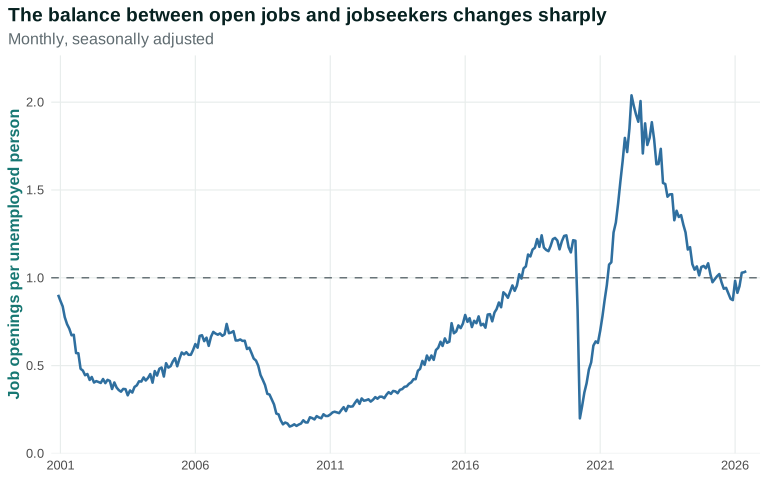
The balance changes markedly. During weak labor markets the ratio is far below one. It rises above one before the pandemic, drops abruptly in 2020, and then climbs to an unprecedented level in this series.
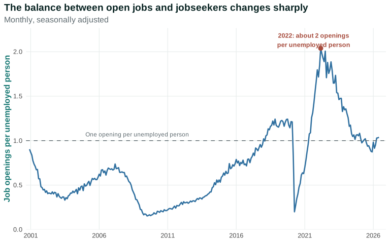
The 2022 annotation establishes timing, not a complete explanation. Hiring demand, labor-force participation, sectoral reallocation, illness, care responsibilities, migration, wages, and working conditions can all affect the numerator, the denominator, and whether a match occurs.
Everyday Economics 3.1
What does “shortage” mean?
A vacancy can coexist with applicants if the wage and conditions do not create an acceptable match. What would persuade a worker to accept? What would persuade the employer to improve the offer?
One vacancy is not the aggregate labor market, and the aggregate ratio is not a universal law about any vacancy. Together, the restaurant story and the data identify actors, goals, constraints, and feedback that the model must organize: why can vacancies and unemployment coexist, how do firms respond, and what do wages and prices have to do with the outcome?
The restaurant has several possible responses, and each response has a constraint.
| Possible response | What the employer hopes to accomplish | Constraint or consequence |
|---|---|---|
| Raise the wage | Attract applicants or reduce quits | Labor cost rises unless productivity, prices, or another margin changes |
| Improve schedules or conditions | Make the job more attractive and improve retention | May require more staffing, coordination, or managerial change |
| Leave shifts vacant | Avoid accepting a higher wage bill | Output, service quality, and customer relationships may suffer |
| Redesign work or buy equipment | Produce with fewer labor hours | Requires time and investment and may change the jobs that remain |
| Raise menu prices | Cover some increase in nominal costs | Customers may buy less or switch to another restaurant |
This table supplies the bridge to the rest of the chapter. Chapter 2 explained why labor-market conditions can change the wage firms find it useful or necessary to offer. It did not explain how much output a worker produces, how the firm sets its product price, or how wages and profits fit within the revenue generated by that output. To connect a pay increase to a real wage—what the money wage can buy—we need to add customers, productivity, costs, prices, and ownership to the story.
Reporting flag: Add a named US employer-worker case only after verifying the timeline, local labor-market conditions, wage measure, and alternative explanations. Verify the JOLTS opening definition and the CPS unemployment denominator; avoid treating either a quote or the national ratio as representative of every occupation and place.
Questions
Review the live step-by-step figure
Question 3.1. In Figure 3.1, what does a ratio of two job openings per unemployed person mean?
- Every unemployed person has received two acceptable offers
- The national count of reported nonfarm openings is twice the number of people classified as unemployed
- Every employer must double wages
- Unemployment has fallen to zero
Exercise
One help-wanted sign
Use Figure 3.1 to compare a month when the openings-to-unemployed ratio is below one with the 2022 peak. Explain why neither the national ratio nor one vacancy proves a shortage for a particular restaurant. Name two worker-side and two firm-side facts you would want before explaining the outcome.
The model solution is available in the restricted instructor materials.
3.2 The employment contract is incomplete
An incomplete contract cannot specify and enforce every action each party will take in every circumstance. A job description can state hours and tasks, but it cannot list every moment in which a worker should use judgment, help a colleague, solve a problem, or choose how carefully to work.
This creates a principal–agent problem. The employer—the principal—wants the worker—the agent—to take actions that contribute to production. Effort is costly to the worker and only partly observable. Monitoring can help, but monitoring is costly and imperfect. UOE Micro Ch. 11
The employment relationship nevertheless creates gains. The firm receives work that helps produce and sell output. The worker receives pay and other benefits. An employment rent is the net benefit of keeping the job compared with the worker’s outside option. If losing the job would be costly, the worker has a reason to meet the employer’s required effort even when every action cannot be enforced.
| Worker receives from job | Worker gives up or bears |
|---|---|
| Wage, benefits, experience, relationships | Effort, time, commute, schedule constraints |
| Continued employment | Risk of discipline or dismissal |
| Employment rent relative to outside option | Opportunities available in the next-best alternative |
The model does not assume that workers are lazy or employers benevolent. It asks what each actor values and which actions are feasible. Norms, professional identity, trust, fairness, and intrinsic motivation may all matter alongside material incentives.
Authority matters as well. During paid hours, an employer usually has the legal and organizational power to assign tasks, evaluate performance, and dismiss a worker within the constraints of contracts and law. A worker can comply, negotiate, organize with coworkers, or leave, but those options have different costs. Someone with savings, portable health insurance, a strong professional network, or another offer can withstand job loss more easily than someone facing rent due, care responsibilities, disability barriers, or restrictions connected to immigration status. These differences change the outside option and therefore the employment relationship itself.
Chapter 2 used this reasoning to build wage setting. We do not need to repeat the entire construction. We need only retrieve the pieces that the new price-setting model must fit.
Imagine that a restaurant worker receives a weekly wage worth 900 units of consumption, gives up time and effort valued at 150, and expects a next-best alternative worth 600 after search costs. The employment rent over that week is \(900 - 150 - 600 = 150\) units. The number is stylized, but the comparison is useful. If job finding becomes easier and the next-best alternative rises to 700, the employment rent falls to 50 unless the employer changes pay, conditions, or the cost of job loss. If a worker’s health insurance is tied to the job, or if dismissal threatens immigration status, the material cost of job loss may be much larger. A single WS curve compresses these unequal positions; it does not erase them.
The employer also faces choices. More monitoring may make performance easier to observe, but supervisors and measurement systems cost money and can damage trust. A higher wage may reduce quits and recruitment costs, but it raises the wage bill. Better scheduling can make the job more attractive without changing the hourly wage, but predictable schedules may require additional staff. The firm chooses a package rather than one number in isolation. The model uses the real wage as a summary because it is one important and measurable part of that package.
Questions
Question 3.2. What makes an employment contract incomplete?
- It never states a wage
- It cannot specify and enforce every worker action in every circumstance
- It lasts less than a year
- It is not written on paper
Exercise
What the contract leaves out
Choose a job and list three valuable worker actions that would be difficult to specify and enforce completely. Explain how monitoring, norms, and the cost of job loss might affect one action.
The model solution is available in the restricted instructor materials.
3.3 What wage setting brings forward from Chapter 2
Chapter 2 built wage setting from feasible offers. The firm wants to recruit, retain, and motivate workers while controlling costs. The worker values income and job security but also values time and finds effort costly. The firm cannot simply choose the lowest possible wage: a very low wage may cause vacancies, quits, or insufficient effort.
The Doing the best you can principle therefore applies to both sides. A firm chooses a wage it believes will produce the most valued feasible outcome given recruitment and motivation constraints. A worker chooses effort given the wage, monitoring, norms, and consequences of losing the job.
Unemployment affects the outside option. When unemployment is high and job finding is difficult, losing a job is more costly. When the labor market is tight and another job is easier to find, a firm may need to offer a higher real wage to create the same employment rent. The wage-setting curve carries this relationship forward: it records the feasible real wage at each employment level. TE 2.0 §1.6
The wage-setting curve is a behavioral relationship, not an accounting identity. Its position depends on institutions and behavior. We now hold it in place temporarily and ask a new question: what real wage is consistent with firms’ price choices? Only after building that second constraint will we bring the two together.
| What Chapter 2 established | Meaning carried into Chapter 3 | What it does not yet determine |
|---|---|---|
| Employment contracts are incomplete | Pay, authority, monitoring, trust, and job-loss costs can affect retention and effective work | The product price or profit per worker |
| Workers have outside options | Easier job finding generally makes losing the current job less costly | Whether a higher nominal wage becomes a higher real wage |
| Firms choose feasible wage offers | The useful offer need not be the lowest possible wage | How much revenue is available to cover wages and profits |
| WS rises with employment in the simplified model | Tighter labor markets require a higher real wage for wage-setting plans to work | Which employment and real-wage combination is mutually consistent |
The last column is the reason for price setting. A wage-setting plan can tell an employer what wage may recruit and retain workers at a given employment level. The firm must also sell what those workers produce. If the money wage rises while product prices rise just as much, the real wage does not rise. If productivity increases, more output is available per worker. If market power permits a larger markup, owners may receive a larger share while the price-setting real wage falls. We need a second relationship to organize those possibilities.
Everyday Economics 3.2
Why not pay the lowest wage?
Think of a job with costly turnover or difficult-to-observe quality. How could a higher wage save the employer money or improve the product?
Questions
Review the live step-by-step figure
Question 3.3. Why does a tighter labor market tend to raise the wage-setting curve?
- Jobs become harder to find
- Losing a job becomes less costly, so firms need a larger employment rent
- Productivity must fall
- Prices are legally fixed
Exercise
Build an employment rent
A job pays $900 per week and requires effort valued by the worker at $150. The next-best alternative provides $500 after search costs. Calculate the weekly employment rent and predict how a better outside option changes the wage needed to motivate effort.
The model solution is available in the restricted instructor materials.
3.4 Micro tools for price setting
Firms also interact with customers. A firm’s demand curve describes how many units customers will buy at alternative prices, holding relevant conditions fixed. Producing another unit creates marginal cost. A firm with some market power weighs the gain from a higher price against the loss of sales. If close substitutes are available, a price increase may lose many customers. If substitutes are scarce, the firm has more room to set price above cost.
Consider two restaurants with the same kitchen technology and wage. One sits on a block with several close substitutes; the other is the only late-night option near a highway exit. A price increase at the first restaurant may move many customers to a rival. The second may lose fewer. The difference does not mean that the second firm can charge any price it wants. Customers can still cook, travel farther, change what they buy, or stop buying. Market power is room to choose within constraints, not the absence of constraints.
The firm’s product demand and cost therefore play different roles. Demand describes customers’ responses to alternative prices. Cost describes what the firm gives up to produce and sell another unit. Profit is revenue minus costs. A profit-seeking firm evaluates the entire consequence of a price: the margin earned on each unit and the number of units it expects to sell. For this chapter, we do not solve that optimization problem algebraically. We use its consequence—a markup—and ask how it constrains the real wage economy-wide.
UOE Micro Chapters 12–14 build this logic from willingness to pay, costs, demand, and profit. For the macro model, we retain only the bridge: firms set prices above marginal cost when they have market power, and the feasible gap depends on how customers respond and how intense competition is. UOE Micro Chs. 12–14
A markup is the gap between price and cost, expressed in a declared way. If unit labor cost is $0.80 and price is $1.00, the dollar markup is $0.20. In this chapter, we express the markup as a percentage of unit labor cost: \((1.00 - 0.80)/0.80 = 25\%\). The same gap is 20% of the price, which is why stating the convention matters.
To see the firm-level choice before drawing a macroeconomic curve, suppose one worker produces 20 meals in the model period. Labor is the only variable production cost in this first example. The table reports values in dollars and then translates the wage into units of the firm’s product.
| Quantity | Value | How to read it |
|---|---|---|
| Output per worker | 20 meals | Productivity in the model period |
| Price | $1 per meal | The chosen unit makes the arithmetic transparent |
| Unit labor cost | $0.80 per meal | Wage cost associated with each meal produced |
| Nominal wage per worker | $16 | 20 meals × $0.80 |
| Real wage | 16 meals | $16 divided by $1 per meal |
| Profit per worker | $4 | $20 revenue minus the $16 wage |
| Markup | 25% of unit labor cost | ($1 − $0.80) divided by $0.80 |
The price of $1 is a normalization: it chooses a convenient measuring unit. What matters is the ratio between the nominal wage and the product price. If every dollar value doubled—price to $2 and the wage to $32—the worker would still receive a real wage of 16 meals and the model’s division would be unchanged.
The exact profit-maximizing formula belongs in an optional extension, not in the main path here. The intuition is enough for this chapter: demand constrains the price, production constrains the cost, and competition affects how large a gap the firm can sustain between the two. When many firms make such choices, their prices help determine what a nominal wage can buy.
This example deliberately holds nonlabor inputs aside. Real restaurants buy food, rent buildings, use energy, and pay for equipment and services. Adding those costs would reduce the part of revenue available for wages and profit unless productivity or price also changed. We postpone that extra accounting step because it should not obscure the first connection between productivity, the markup, and the real wage.
It also matters which costs are fixed and which vary with output. Rent may be due even when the restaurant serves one fewer meal. Ingredients generally change with meals served. Equipment may require a large payment now and lower labor needs later. These distinctions are essential for a full firm model, but the macroeconomic PS curve deliberately compresses them. Its purpose is not to forecast one restaurant’s profit. Its purpose is to connect a common productivity and markup assumption to a feasible real wage.
Do not confuse the demand curve facing one firm with aggregate demand. A firm can lose customers to rivals when it raises its relative price. Aggregate demand concerns total planned spending across the economy and will appear in Chapter 6.
From one firm’s price to economy-wide price setting
The restaurant example describes one firm, yet the PS curve is an economy-wide relationship. Moving between those levels requires an aggregation step. Imagine many firms, each setting a price for its own product. They differ in technology, wages, input costs, customer loyalty, and the competitors they face. A price index combines the prices of many goods and services. The aggregate real wage compares the money wage with that price level. The simple model represents this varied economy as if firms shared a common productivity and markup.
That representation is useful only when we remember what has been compressed. A price increase at one restaurant makes that restaurant more expensive relative to nearby alternatives. If many firms raise prices together, the economy-wide price level rises, and a worker’s money wage buys less across many purchases. The first response mainly redirects demand between firms. The second changes the purchasing power of income. Individual firms do not choose the aggregate price level, but their price choices jointly create it.
The same distinction applies to wages. One employer can raise its wage and recruit from another employer without changing total employment. If employers across the economy try to hire more workers, the resulting competition can strengthen outside options and move the economy along WS. The model connects these decentralized choices through aggregate feedback; it does not imagine a single employer setting the national wage.
Aggregation also warns against a composition mistake. Average productivity can rise because every workplace becomes more productive, because workers move from lower-productivity to higher-productivity activities, or because low-productivity firms close. Those stories may have different consequences for workers even if the same average appears in the graph. Later empirical work must look behind the average before treating a movement in PS as one uniform technological event.
Questions
Question 3.4. What most directly constrains a firm’s price above marginal cost?
- How buyers respond to the price
- The unemployment definition
- The number of retirees
- The base year of the CPI
Exercise
From cost to markup
A firm has marginal cost of $8 and charges $10. Calculate the dollar markup and markup as a percentage of marginal cost. Explain why a steeper demand response could constrain the chosen price.
The model solution is available in the restricted instructor materials.
3.5 Price setting and the feasible real wage
Suppose labor is the only variable input. If a worker produces more output per hour, the firm can pay a higher real wage for a given markup. If firms charge a larger markup for given productivity, a smaller share of output is consistent with wages. The price-setting curve summarizes that feasible real wage. TE 2.0 §1.7
In the simplest version, productivity and competitive conditions are fixed, so the price-setting real wage does not depend on employment. The curve is horizontal. This is an assumption chosen to isolate a mechanism, not a claim that productivity, markups, or competition never change.
The numerical table gives the price-setting real wage directly. A worker produces 20 units, and the 25% markup on unit labor cost is consistent with a real wage of 16 units. Owners receive the remaining 4 units as profit per employed worker. If productivity rises to 24 with the same markup, the price-setting real wage becomes 19.2 units and profit becomes 4.8. If market power instead raises the markup while productivity stays at 20, the price-setting real wage falls.
The language “divides output” describes the model’s outcome, not a meeting in which a firm literally divides a pile of meals. The nominal wage is set in dollars, the firm sets a product price, and their ratio is the real wage. With a larger markup, the price is higher relative to the wage and the real wage is lower. With higher productivity, more output per worker is available to divide.
This point protects us from two common errors. First, higher nominal pay need not mean higher purchasing power. If the wage rises 5% and the prices workers pay also rise 5%, the real wage is unchanged. Second, higher productivity creates room for higher real wages but does not mechanically deliver them. If the markup rises at the same time, some or all of the additional output can appear as profit rather than wages or lower prices. Institutions, bargaining, and product-market competition help determine the division.
The price-setting real wage is feasible under the model assumptions; it is not a legal ceiling or an engineering constant. A firm could temporarily pay more and accept a lower markup, or pay less and earn a higher margin if its wage-setting plan still worked. The PS curve describes the common real wage consistent with the assumed markup when firms have completed their price-setting responses. This conditional language becomes important when we combine PS with WS.
Keep nominal and real changes separate
Suppose the money wage is $16 and the price of the model’s product is $1. The real wage is 16 units. Now compare three cases.
| Changed condition | Money wage | Product price | Real wage | What changed? |
|---|---|---|---|---|
| Baseline | $16 | $1.00 | 16 units | Starting point |
| Wage and price both rise 25% | $20 | $1.25 | 16 units | Nominal values change; purchasing power does not |
| Wage rises while price is fixed | $20 | $1.00 | 20 units | Purchasing power rises; the markup must fall unless productivity changes |
| Productivity rises with the original markup | $19.20 | $1.00 | 19.2 units | More output per worker supports a higher real wage and profit per worker |
The second row is especially important. A worker sees a larger number on a paycheck, but every dollar buys fewer units of the product. The model is therefore stated in real wages. The third row is possible as a temporary firm decision, yet it is not consistent with the original price-setting plan: with unchanged productivity, paying 20 rather than 16 leaves nothing for profit in this example. The final row changes the size of the available output rather than only its dollar labels.
In an actual economy, workers buy a basket of products rather than the output of their own employer. Their real wage therefore depends on a consumer price index, while a firm’s cost calculations depend on the price of its own output and inputs. The simple model treats these prices as moving together. That assumption is convenient for learning the mechanism, but it can be misleading when energy, housing, imported inputs, or particular consumer prices move differently. Chapter 8 will need more detailed price measures when it studies inflation.
Everyday Economics 3.3
Productivity is not automatically pay
More output per hour expands what can be divided. Institutions and market power help determine how much appears as wages, profits, lower prices, or other outcomes.
Reading the price-setting figure one step at a time
The horizontal axis measures employment. The vertical axis must accommodate both output per worker and the real wage because the figure will show how output is divided.
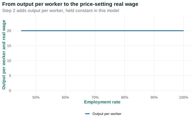
Holding productivity fixed makes output per worker horizontal. This is a simplifying assumption, not a claim that productivity never changes.
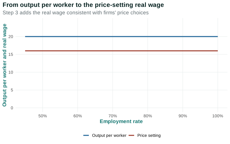
For the assumed competitive conditions, firms’ price choices are consistent with the same real wage at every employment rate.
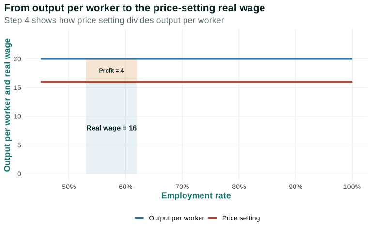
The distance from zero to PS is the real wage. The remaining distance to output per worker is profit per worker in the simplified model. Higher productivity lifts the upper boundary; stronger competition tends to reduce the profit share and raise PS.
Questions
Review the live step-by-step figure
Question 3.5. In the simplified model, what raises the price-setting real wage?
- Lower labor productivity
- A larger markup with unchanged productivity
- Higher productivity with the markup unchanged
- A different label on the vertical axis
Exercise
Productivity and the feasible wage
Compare two economies with the same markup but different output per hour. Use words and a numerical example to show why higher productivity can support a higher price-setting real wage.
The model solution is available in the restricted instructor materials.
3.6 Combining wage setting and price setting
Figure 3.3 places both relationships on common axes. The horizontal axis is the employment rate; the vertical axis is the real wage. At higher employment, unemployment is lower and workers’ outside options are generally better. The wage-setting relationship therefore slopes upward. The price-setting relationship is horizontal in the simplified case.
Reading the combined WS–PS figure one step at a time
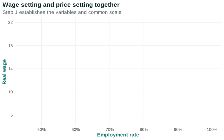
Moving right means more of the labor force is employed and less is unemployed. Moving up means a higher real wage.
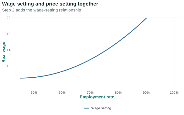
The curve becomes steep as employment approaches the labor-force endpoint: outside options strengthen and creating a sufficient employment rent becomes more costly.
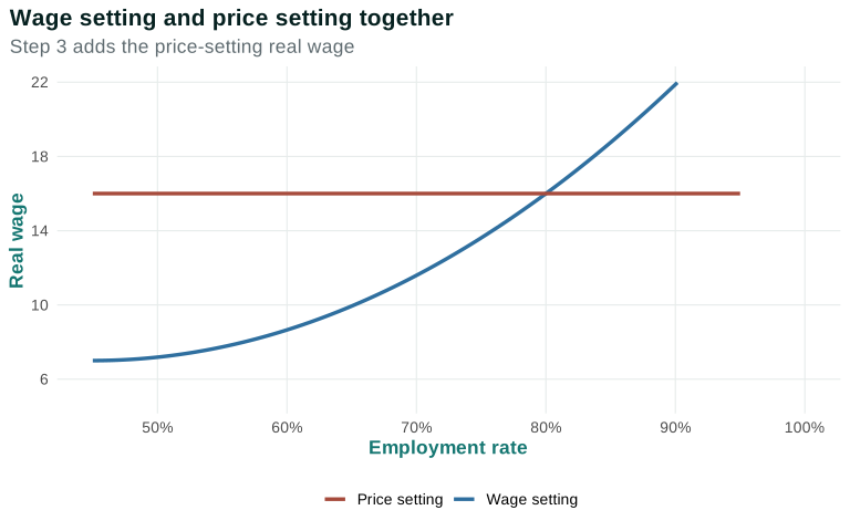
The price-setting curve states the real wage consistent with firms’ prices for fixed productivity and markup.
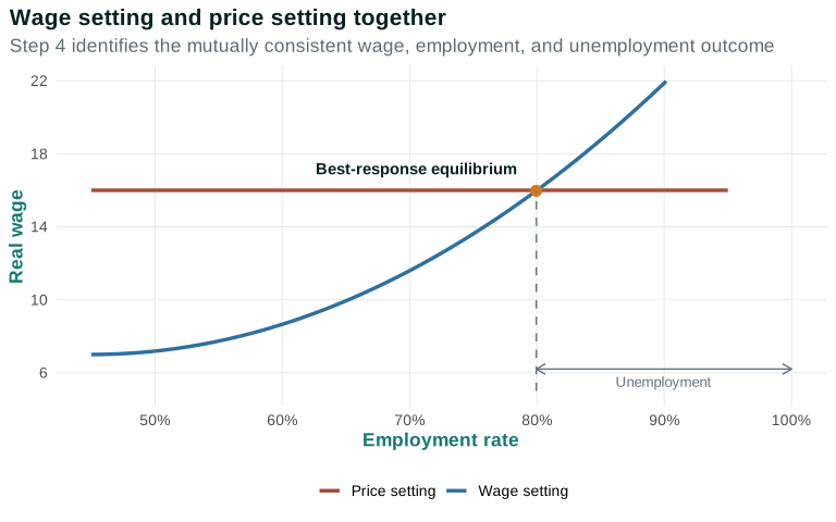
At the intersection, wage-setting and price-setting choices are mutually consistent. The best-response equilibrium includes unemployment: at employment above the intersection, the wage needed to recruit and motivate workers would exceed the real wage consistent with price setting. TE 2.0 §§1.5, 1.8
Test plans away from the intersection
An intersection is more useful when we understand why other points are not mutually consistent. Consider three named situations.
| Situation | Wage-setting plan | Price-setting plan | What is inconsistent? |
|---|---|---|---|
| A: wage below WS | The wage is too low to produce the retention or effective-work response summarized by WS | The wage may be affordable at the stated price | The firm’s labor plan does not work as assumed |
| B: employment to the right of equilibrium | Tight conditions require a real wage above PS | Productivity and markup permit only the PS real wage | The required wage and feasible price-setting wage cannot both hold |
| E: the intersection | The wage is compatible with wage-setting plans | The same wage is compatible with price-setting plans | Neither plan calls for a different real wage under the assumptions |
At A, a firm may experience vacancies, quits, lower effective work, or pressure to improve the offer and working conditions. At B, broad wage pressure may raise nominal labor costs. Firms that protect their markup may raise prices, which erodes the real wage; they may also reduce hiring or output. As employment falls, job finding becomes harder and outside options weaken. These responses point back toward a mutually consistent outcome.
But the diagram does not provide a clock or a unique path. It does not tell us whether nominal wages or prices adjust first, how quickly firms change hiring, or whether customers buy the output firms would like to sell. Those questions require aggregate demand, expectations, contracts, and policy. Chapter 6 will add the spending–income feedback needed to analyze output and employment adjustment more fully. Here the intersection is first a compatibility test: it identifies the real wage and employment level at which the two plans fit.
Unemployed workers cannot necessarily obtain jobs by offering to work for less. A firm that paid a wage too low to create the required employment rent would not believe that effort could be sustained merely because a worker promised it. The equilibrium is not socially ideal by definition; it is an outcome in which individual best responses are mutually consistent.
This unemployment is involuntary unemployment: people would prefer employment at the going real wage but do not have jobs. The result differs from a simple auction story in which a lower offer always secures a sale. Labor is performed over time inside an incomplete contract. The wage affects retention, effort, cooperation, and the value of keeping the job. An individual promise to work for less does not remove the firm’s concern that the relationship must remain effective after hiring.
Nor does equilibrium mean that every worker and firm is satisfied. An unemployed person may face severe hardship. A worker may dislike the wage, schedule, or authority relationship. An employer may want a larger margin. “Best response” means that, given the other conditions and available actions represented in the model, an actor does not have a feasible alternative that produces a more valued modeled outcome. Change the rules, outside options, technology, or market structure and the best responses can change.
This mutual dependence is the Principle of aggregation and feedback. Each firm responds to economy-wide unemployment and prices. All firms’ wage, price, hiring, and output choices together create those aggregate outcomes.
Read equilibrium as a conditional claim
The word equilibrium can sound as though the economy is peaceful, fair, or motionless. None of those meanings follows. In this chapter it means that two modeled plans are compatible under a stated set of conditions. A useful way to read the intersection is as a sequence of conditional questions:
- At this employment level, what real wage does wage setting require for firms’ recruitment and effective-work plans to succeed?
- Given productivity and the markup, what real wage is consistent with firms’ price-setting plans?
- Do those two answers match?
At \(E\), they match. Away from \(E\), at least one plan calls for a different wage, price, or employment level. This is why simply naming the intersection is not enough; students should be able to explain which actor would reconsider which choice at a named off-equilibrium point.
The conclusion is conditional in another sense. If unemployment insurance, monitoring technology, discrimination, union organization, or job-search institutions change, WS may change. If productivity, input costs, or product-market competition change, PS may change. The old intersection does not remain a prediction after a condition changes. We must rebuild the comparison with the changed relationship.
Finally, the intersection summarizes averages. Two workers can have different outside options at the same unemployment rate. Two firms can face different customer demand and markups at the same aggregate price level. An aggregate equilibrium can coexist with vacancies in one place, layoffs in another, high employment rents for some workers, and weak bargaining positions for others. The model gives a disciplined starting point, not permission to ignore those differences.
Questions
Review the live step-by-step figure
Question 3.6. What is true at the WS–PS intersection?
- Unemployment is necessarily zero
- Wage-setting and price-setting choices are mutually consistent
- Every worker and firm receives the same income
- No institution affects the outcome
Exercise
Read the equilibrium
Use Figure 3.3 to identify the equilibrium real wage and employment conceptually. Then explain why unemployed workers cannot necessarily obtain jobs simply by offering to work for less.
The model solution is available in the restricted instructor materials.
3.7 Productivity, competition, and labor-market tightness
We can now change one condition at a time and trace whose choices respond.
Higher productivity. Suppose redesigned work or better equipment raises output per worker from 20 to 24 units while the markup stays at 25%. Firms can sustain a higher real wage at every employment level, so PS moves upward. The new intersection has a higher real wage and, in this simplified model, more employment. More output makes a larger total gain possible; it does not guarantee how every worker or owner shares it when markups and bargaining also change.
A larger markup or weaker competition. Suppose customers have fewer close alternatives, allowing firms to charge a larger price relative to unit labor cost. With productivity fixed, PS moves downward. The real wage consistent with price setting falls, and the intersection moves to lower employment. Owners receive a larger share per unit in the simplified accounting, while workers face lower purchasing power and greater unemployment risk.
A stronger worker outside option. Suppose unemployment insurance becomes more protective, another employer enters the local market, or collective organization makes job loss less damaging. At any given employment level, a firm may need to offer a higher real wage to recruit or retain workers, so WS moves upward. With PS unchanged, the new intersection lies at lower employment. Chapter 4 will show why institutions can also affect voice, turnover, productivity, and PS; those channels must be analyzed separately.
A tighter labor market with both relationships unchanged. Moving right along the existing WS curve is not a change in the conditions underlying WS. It is a comparison between two employment levels on the same relationship. The distinction matters because a movement along WS and a changed outside-option institution answer different questions.
Compare named outcomes in a fixed order
When a condition changes, avoid jumping from “the curve shifts” to a conclusion. Use the same reading order each time. First name the condition held fixed. Second identify the actor whose feasible choice changes. Third move the relevant relationship. Fourth locate the new intersection. Finally compare the real wage, employment, unemployment, and division of output at the two named points.
For example, begin at \(E\) with productivity of 20, a real wage of 16, and 80 employed people. If productivity rises to 24 while the markup and WS relationship remain fixed, the firm can offer a higher price-setting real wage at every employment level. PS rises to 19.2. The new intersection must be above and to the right of \(E\) in this stylized model: both the real wage and employment rise, while unemployment falls. The numerical labels make the direction visible; the exact new employment number depends on the particular WS curve.
Now return to \(E\) and instead allow a larger markup while productivity stays at 20. PS falls. The new intersection is below and to the left: the real wage and employment fall, while unemployment rises. This is not the same as observing a fall in employment and declaring that a markup caused it. The diagram gives a conditional prediction. Establishing a historical cause requires evidence that the markup changed first, that productivity and other relevant conditions were adequately addressed, and that the timing and magnitude fit the proposed mechanism.
The fixed reading order is a form of scaffolding. It lets students check each inference and helps prevent contradictory claims—for example, moving WS but reporting a change that would require PS to move as well.
The effects also distribute risk differently. A productivity increase can make both a higher wage and higher profit possible, but investment costs and job redesign may expose some workers to displacement. A larger markup transfers purchasing power away from wages in the simplified model and may reduce employment. A stronger outside option protects workers who lose jobs or reject poor offers, while firms face a higher cost of recruiting and retaining labor. The model clarifies these conditional pressures; evidence and institutional detail determine their size and who actually bears them.
Some conditions can change more than one relationship. A training system can strengthen a worker’s outside option and raise productivity. A union can change bargaining, voice, turnover, and workplace investment. A minimum wage can constrain an employer with wage-setting power while also affecting prices, hiring, or productivity. We analyze one channel at a time so that the logic remains visible, then combine channels only when evidence justifies doing so. Chapter 4 uses exactly this discipline.
These are model predictions under stated assumptions. Real economies add aggregate demand, matching, investment, expectations, policy, worker and firm differences, and adjustment over time. When the data move differently from the prediction, the right response is to investigate which assumption or omitted mechanism matters.
Data Extension 3.7: Productivity, real compensation, and unemployment
The analytical diagram helps organize stories. It does not tell us which story explains a historical episode. This extension combines three pinned BLS series: output per hour in the nonfarm business sector, average real hourly compensation in that sector, and the national unemployment rate.
Read the evidence as three different measures
The upper panel uses an index, so 100 marks the value in 1973 rather than dollars or units of output. The lower panel uses a percentage. Alignment permits comparisons in time; it does not make an index point equal to a percentage point.
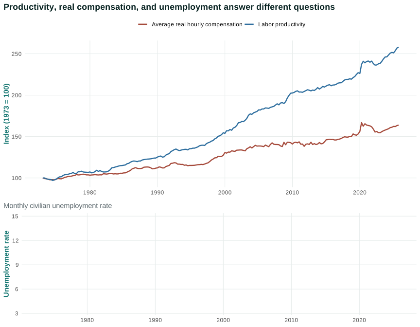
Start with description. Productivity and average real compensation both rise over the long period, but the gap between their indexes changes. The comparison does not by itself identify a cause or describe the median worker.
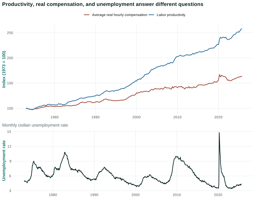
Unemployment moves much more sharply over business-cycle episodes. These patterns are compatible with several mechanisms: productivity can alter PS; markups and the wage/profit division can affect how productivity appears in compensation; labor-market conditions and institutions can affect WS.
Open the live step-by-step figure
Now separate description from explanation. Average compensation includes employer-paid benefits and is not the median worker’s wage, disposable income, or take-home pay. National unemployment compresses large differences across groups and places. None of these series directly observes a WS or PS curve. A serious explanation would add evidence on prices, markups, labor shares, vacancies, institutions, and the timing of decisions.
Intermediate preparation: cost per unit of output
Economists sometimes summarize compensation relative to productivity with unit labor cost: labor compensation associated with producing one unit of output. If compensation grows faster than productivity, unit labor cost rises; if productivity grows faster, it falls. The label is useful in later inflation analysis, but it is a ratio—not a complete theory of prices or wages.
The extension’s task is diagnosis rather than curve spotting: choose a named period, describe all three measures, propose one WS story and one PS story, and state what additional evidence would distinguish them.
Questions
Review the live step-by-step figure
Question 3.7. Which change most directly shifts the price-setting relationship upward?
- Higher labor productivity
- A higher cost of job loss
- Lower unemployment with curves unchanged
- More active job search
Exercise
Shift one relationship
For higher productivity, weaker product-market competition, and more generous unemployment insurance, state which relationship shifts first and trace the predicted changes without assuming other mechanisms are absent.
The model solution is available in the restricted instructor materials.
3.8 What the model explains—and leaves out
The WS–PS model is an institutional map. It connects incomplete contracts and employment rents in the labor market with demand, costs, and markups in product markets. It explains why persistent unemployment can coexist with optimizing workers and firms, and it provides disciplined predictions about changes in productivity, competition, and outside options.
Return to the composite restaurant. A help-wanted sign and a high openings-to-unemployed ratio can strengthen workers’ alternatives and put upward pressure on offers. Whether the resulting nominal pay becomes a higher real wage depends on output per worker, prices, and the markup. Leaving the vacancy open sacrifices output; raising the wage changes cost; raising the price tests customer demand; redesigning work changes productivity. The model does not select one response without further facts, but it prevents us from explaining the outcome with a single actor’s preferences.
It also keeps four kinds of reasoning distinct. The division of output per worker is an accounting relationship. WS and PS are behavioral/model relationships. Claims that a historical institution caused a wage or employment change require evidence beyond the diagram. And the feedback from many firms’ choices to economy-wide unemployment and prices is an aggregation mechanism. Confusing these categories is a common source of weak macroeconomic arguments.
It leaves out much that matters: job matching, occupations, discrimination, unions as strategic actors, household care constraints, varying productivity, multiple products, aggregate demand, inflation dynamics, finance, and policy adjustment. Later chapters add these mechanisms rather than asking one diagram to explain the whole economy.
The next chapter makes distribution explicit. It asks who receives wages and profits, how unemployment changes the distribution of market income, and how collective bargaining, voice, competition, and public rules can change both the size and division of economic gains.
The handoff is numerical as well as conceptual. Chapter 4 begins with the same 20 units of output per worker, 16-unit real wage, 4 units of profit per worker, and 80 employed people used here. Holding that baseline fixed means that any later change in the income distribution can be traced to a declared change in employment, productivity, bargaining, or the markup rather than to an unnoticed recalibration.
Seeing the principles in action
| Principle | Example | Everyday Economics |
|---|---|---|
| Interdependence principle — focal | Workers’ effort depends on wages and outside options; firms’ wage and price choices depend on what other firms and workers do. | An employer’s pay decision changes when nearby employers raise wages and workers can leave more easily. |
| Doing the best you can principle — focal | Workers choose effort given the cost of effort and job loss; firms choose wages and prices subject to recruitment, motivation, demand, and cost constraints. | Paying the lowest possible wage may not maximize profit if it causes quits or low effort. |
| Rules of the game principle | Employment protection, unions, minimum wages, unemployment insurance, and product-market regulation change outside options and feasible markups. | A change in unemployment insurance can alter the cost of job loss and therefore the wage-setting relationship. |
| Trade-offs and opportunity costs principle | Higher effort is costly to workers, while a higher wage raises a firm’s cost but can increase the value of keeping the job. | A worker compares the benefit of conserving effort today with the risk and cost of losing the job. |
| Principle of gains from cooperation and conflict of interest | Employment produces output and income that benefit workers and firms, but they have conflicts over effort, wages, prices, and the division of output. | A profitable employment relationship can still involve bargaining over schedules and pay. |
| Principle of individual and societal interests | Profit-seeking wage and price decisions can be mutually consistent while leaving some willing workers without jobs. | No individual firm may want to hire at a lower wage even though unemployed workers would prefer employment. |
| Principle of aggregation and feedback — focal | Each firm’s wage and price responds to economy-wide unemployment and prices, while all firms’ choices together create those aggregate outcomes. | A wage increase at one firm is local; similar increases across firms can also affect costs, prices, and the real wage. |
Skills and learning objectives
- Translating a story into an abstract model
- Reading an analytical graph
- Interpreting a graph with multiple curves
- Adjusting a model in response to economic or institutional changes
- Explaining a causal mechanism
- Defining important economic terms
- Applying principles to a specific scenario
Concepts to learn
- Incomplete contracts and principal–agent problems
- Employment rents, outside options, and worker effort
- Wage setting and the wage-setting curve
- Demand facing a firm, marginal cost, price, and markup
- Price setting and the price-setting curve
- Best-response equilibrium and equilibrium unemployment
- Comparative statics, adjustment, and model limitations
Glossary
Chapter 3 terms
incomplete contract
A contract that cannot specify or enforce every action each party will take in every possible circumstance.
See also: principal–agent problem; employment rent.
principal–agent problem
A problem created when a principal wants an agent to take an action that is costly to the agent and cannot be fully observed or enforced.
See also: incomplete contract; employment rent.
employment rent
The net benefit a worker receives from keeping a job compared with the worker’s next-best alternative.
See also: outside option; incomplete contract.
outside option
The next-best alternative available if a current interaction or agreement ends.
See also: employment rent.
wage-setting curve
The real wage firms need to offer at each economy-wide employment level to recruit, retain, and motivate workers.
See also: price-setting curve; best-response equilibrium.
markup
The gap between a firm’s price and its marginal cost, often expressed relative to marginal cost or price.
See also: price-setting curve.
price-setting curve
The real wage consistent with firms’ price-setting choices for given productivity and competitive conditions.
See also: wage-setting curve; markup; best-response equilibrium.
best-response equilibrium
An outcome in which each actor’s action is a best response to the actions and conditions created by others.
See also: wage-setting curve; price-setting curve.
involuntary unemployment
A situation in which people would prefer employment at the going real wage but do not have jobs, and cannot necessarily obtain them simply by offering to work for less.
See also: best-response equilibrium; incomplete contract; employment rent.
Flashcards
What makes an employment contract incomplete?
Not every action or circumstance—especially worker effort—can be specified, observed, and enforced.
Why does lower unemployment tend to raise the wage needed to motivate workers?
Jobs are easier to find, so losing the current job is less costly and firms must offer a larger employment rent.
What determines the price-setting real wage in the simplified model?
Labor productivity and the markup created by firms’ price-setting choices.
What does the WS–PS intersection represent?
A best-response equilibrium where economy-wide wage-setting and price-setting choices are mutually consistent.
Questions
Question 3.8. Which is a limitation of the basic WS–PS model?
- It distinguishes wage setting from price setting
- It compresses worker, firm, and job differences into aggregate relationships
- It contains an equilibrium concept
- It can be drawn as a graph
Exercise
Evaluate the model
Write one outcome the WS–PS model organizes well, one important omission, and one empirical comparison that could test a claim made using the model.
The model solution is available in the restricted instructor materials.